Category Archives: MODIS

Fog over the Ozarks and southern Plains

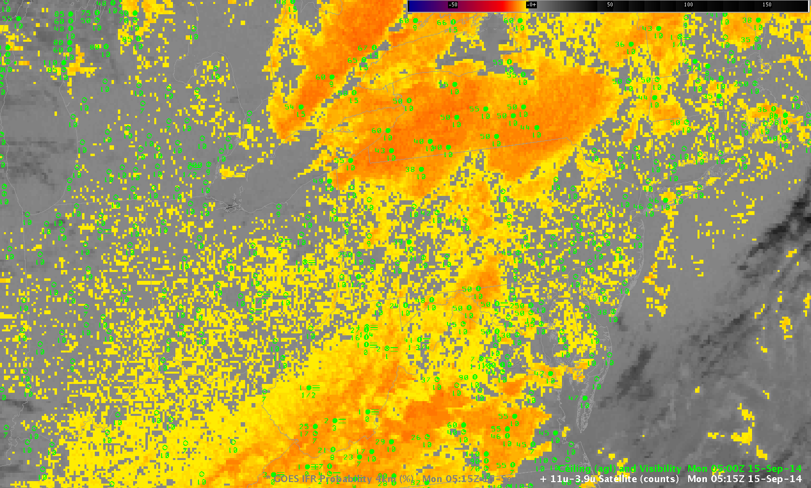
GOES-IFR Probabilities, computed from GOES-13 and Rapid Refresh, hourly from 0100 through 1300 UTC on 21 October 2014 (Click to enlarge)

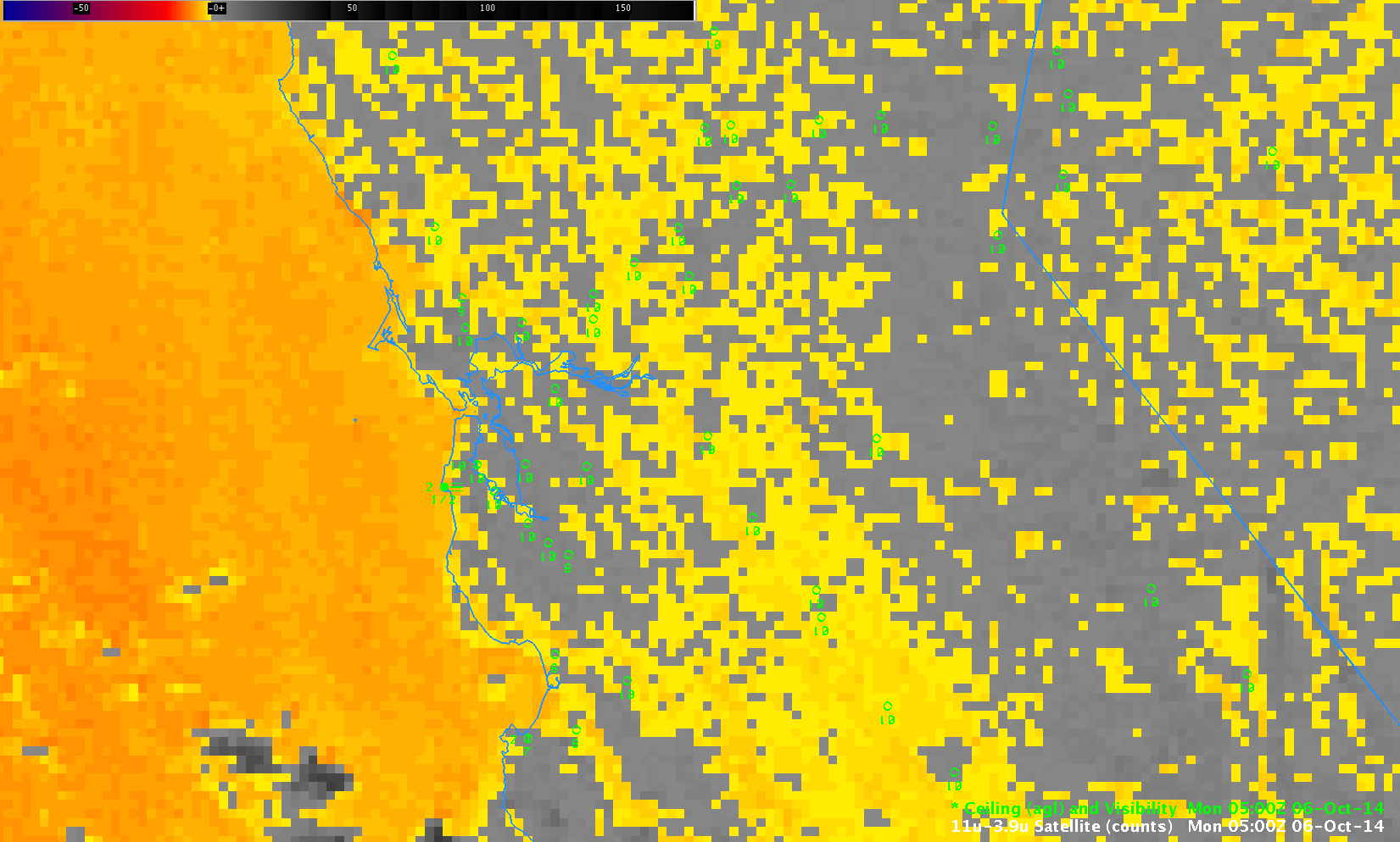
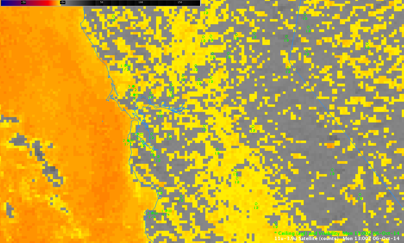
Fog and stratus developed overnight over the Ozark Mountains and southern Plains. The hourly loop of GOES-R IFR Probabilities shows the development and expansion of visibility and ceiling reductions over the area. How do these fields compare to other measures of fog? Brightness Temperature Difference fields, below, generally overestimate the regions of fog. The 0200 and 0800 UTC brightness temperature difference fields, below, are toggled with the IFR Probabilities; the inclusion of surface information via the Rapid Refresh Model correctly limits the positive brightness temperature difference to regions where fog and low stratus are most likely. The satellite-only signal overpredicts regions of reduced visibilities because it can only see the top of the cloudbank; this offers little information about the cloud ceilings!

GOES-13 Brightness Temperature Difference (10.7 µm – 3.9 µm) and GOES-based IFR Probabilities at 0200 UTC, 21 October 2014 (Click to enlarge)

GOES-13 Brightness Temperature Difference (10.7 µm – 3.9 µm) and GOES-based IFR Probabilities at 0800 UTC, 21 October 2014 (Click to enlarge)

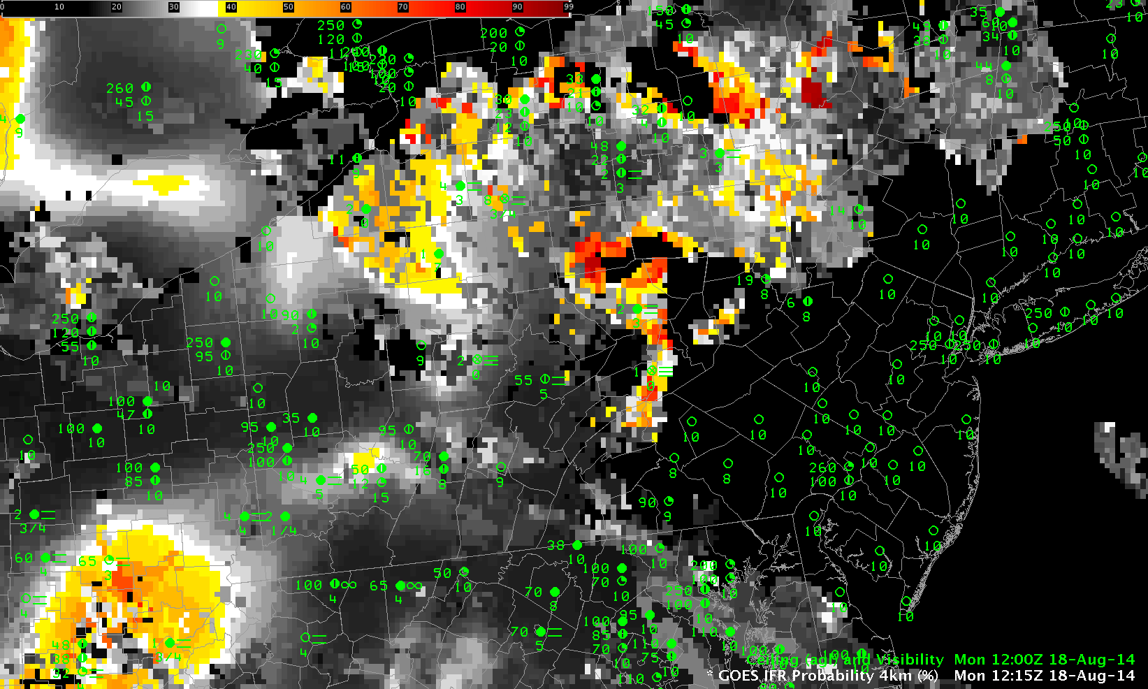
Brightness Temperature Difference fields are occasionally contaminated by stray light in the signal. This happened on 21 October at 0400 UTC. The Brightness Temperature Difference fields at 0345, 0400 and 0415 UTC are shown below, with the GOES-R IFR Probabilities for the same time follow. Note how Stray Light contamination does bleed into the GOES-R IFR Probability field; if there is a large change over 15 minutes in the IFR Probability signal, consider the possible reasons for that change. Stray light contamination is a strong candidate if the signal is near 0400-0500 UTC with GOES-East. There are regions in the IFR Probability fields where even the strong — but meteorologically unimportant — brightness temperature difference signal during stray light is not enough to overcome the information from the Rapid Refresh model that denies the possibility of low-level saturation (for example, in northern Kansas or southern Oklahoma).

GOES-13 Brightness Temperature Difference (10.7 µm – 3.9 µm) at 0345, 0400 and 0415 UTC, 21 October 2014 (Click to enlarge)

GOES-based IFR Probabilities at 0345, 0400 and 0415 UTC, 21 October 2014 (Click to enlarge)

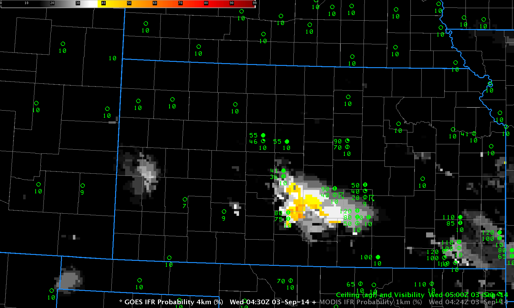
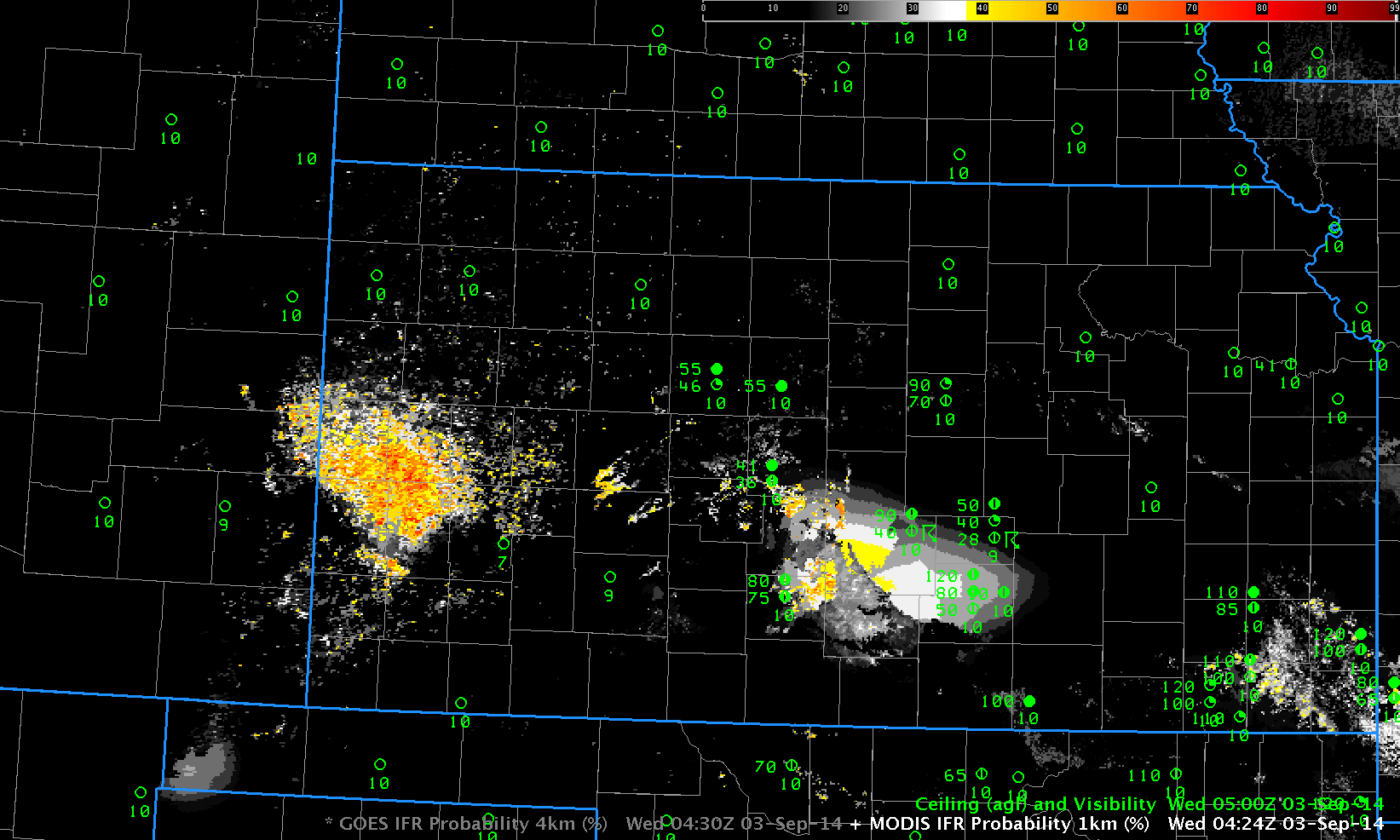
MODIS data from either Terra or Aqua can give important early alerts to the development of Fog/Low Stratus. Because of its superior resolution to GOES, the character of the developing fog can be depicted with more accuracy. The MODIS-based IFR Probability, below, in a toggle with the GOES-based IFR Probability at the same time, distinctly shows that the fog development at 0430 UTC is starting in the small valleys of the Ozarks of northwest Arkansas. GOES-based IFR Probabilities give a broader signal; certainly if you are familiar with the topography of the WFO you can correctly interpret the coarse-resolution GOES data, but the MODIS data spares you that necessity.

GOES- and MODIS-based IFR Probabilities at ~0430 UTC, 21 October 2014 (Click to enlarge)

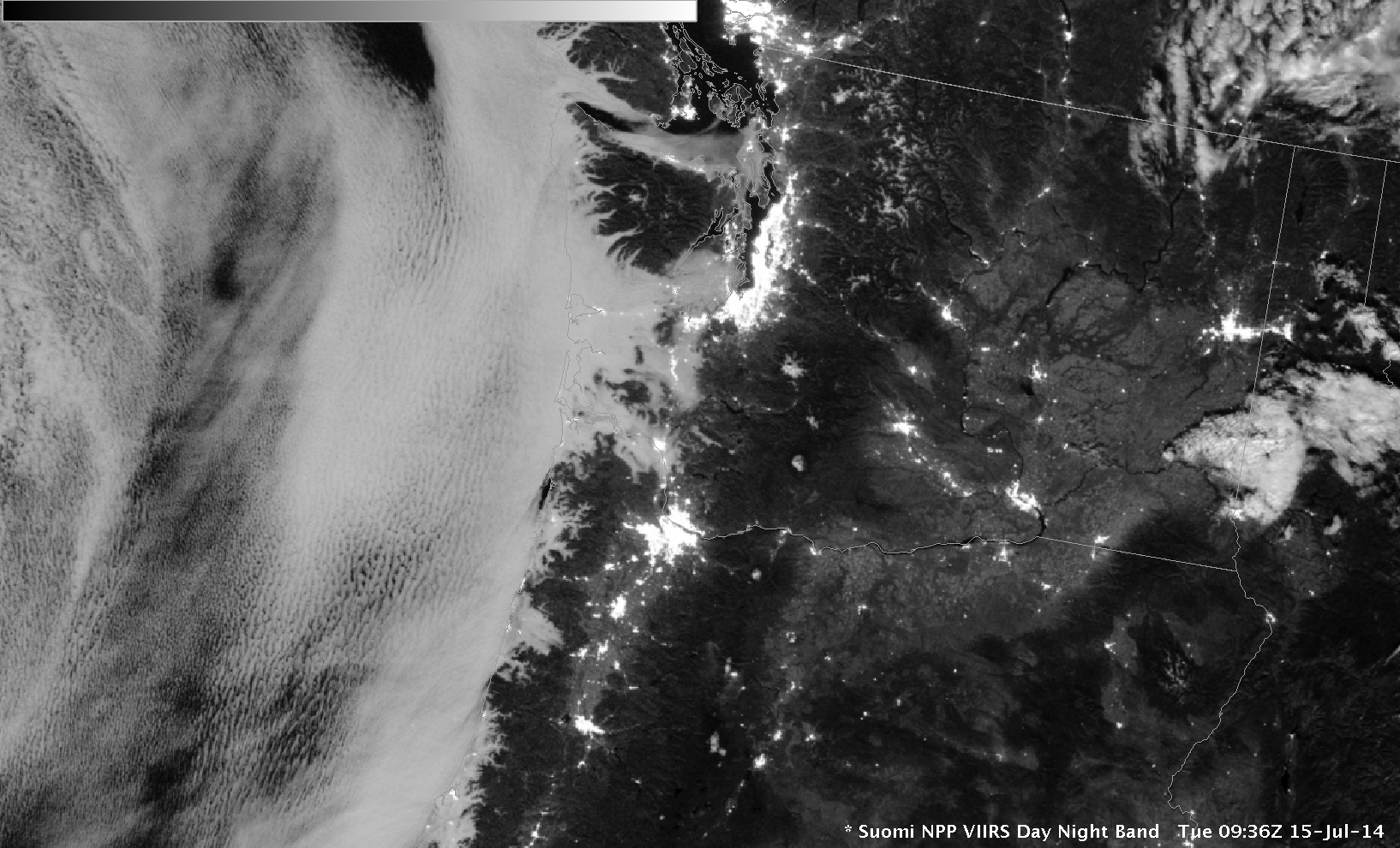
Suomi NPP data can also be used to compute IFR Probabilities, but those data are not yet computed for AWIPS. The Ozarks were properly positioned on 21 October to be scanned by two successive orbits of Suomi NPP (one of the benefits of Suomi NPP’s relatively broad scan), and the brightness temperature difference fields (11.45µm – 3.74µm) at 0715 and 0900 UTC are shown below. As with MODIS, the strong signal in the river valleys is apparent. (The Day Night band from Suomi NPP for this event does not show a strong signal because the near-new Moon provides no illumination at 0745 or 0900 UTC: it hasn’t even risen yet.)

Suomi NPP Brightness Temperature Difference (11.45 µm – 3.74 µm) and 0715 and 0900 UTC, 21 October 2014 (Click to enlarge)

Successive Suomi NPP Scans Show Stratus/Fog movement

Suomi NPP Day/Night Band at 0926 and 1106 UTC on 9 October 2014 (Click to enlarge)

(A Blog post on Suomi NPP Imagery over the western US from 10 October is available here).

Polar orbiters typically don’t give good temporal resolution, especially near the Equator. In mid-latitudes, however, Polar Geometry can yield views over a wide area on two successive scans. This happened along the West Coast early in the morning on 9 October. Two regions show noticeable changes in stratus between the two times: stratus/fog extends farther down the Salinas Valley at the southern edge of image, and stratus/fog expands over southwestern Puget Sound in Washington. The Brightness Temperature Difference field (11.35µm – 3.74µm) from Suomi NPP for the same times shows a similar evolution over the Salinas Valley, but the view of Washington is obscured by thin cirrus. These cirrus (that show up as black enhancements below) are mostly transparent in the Day Night Band but not in the infrared bands.

Suomi NPP Brightness Temperature Difference (11.35µm – 3.74µm) at 0926 and 1106 UTC on 9 October 2014 (Click to enlarge)

MODIS instruments onboard Terra and Aqua yield spectral data that can be used to generate GOES-R IFR Probability Fields. The animation below shows high-resolution imagery of where IFR Probabilities are highest, but only at three distinct times: 2152 UTC on 8 October and 0537 and 0949 UTC on 9 October. An increase in IFR Probabilities around Monterey Bay is apparent (and consistent with the Suomi NPP Observations above); IFR Probabilities also increase along the Oregon Coast and around Puget Sound.

MODIS-based GOES-R IFR Probabilities at 2152 UTC 8 October, 0547 UTC 9 October and 0949 UTC 9 October (Click to enlarge)

How do GOES-based observations complement the Polar Orbiter data above?

GOES-15 based GOES-R IFR Probabilities, hourly from 0200 through 1400 UTC, 9 October 2014 (Click to enlarge)

The hourly animation above shows the slow increase of IFR Probability in/around Monterey Bay, and also a push of higher IFR Probability onto the Oregon Coast that occurs after the last MODIS-based IFR Image shown farther up. (Higher IFR Probabilities also spill into San Francisco Bay). Do surface observations of ceilings and visibilities agree with the IFR Probability fields? The loops below, from Oregon (below) and Monterey Bay (bottom) suggest that they do. For example, Eugene OR (and stations north and south of Eugene) show IFR conditions as the high IFR Probability field moves in after 1100 UTC. GOES-based data is valuable in monitoring the motion of IFR Probability fields; keep in mind, though, that small-scale features may be lost. For example, it is difficult for GOES to resolve the Salinas Valley.

GOES-15 based GOES-R IFR Probabilities, hourly from 0200 through 1500 UTC, 9 October 2014, with surface and ceiling observations superimposed (Click to enlarge)

GOES-15 based GOES-R IFR Probabilities from 0400 through 1400 UTC, 9 October 2014, with surface and ceiling observations superimposed (Click to enlarge)

IFR Probability along the West Coast

MODIS data from Terra and Aqua, Suomi NPP data, and GOES-15 data yield different types of information that can be used to observe clouds in a region. Probabilities of IFR conditions — that is, what’s going on at cloud base, which is a part of the cloud the satellite cannot see — can be produced by combining satellite observations of cloud tops and data from a model (such as the Rapid Refresh) that includes accurate predictions low-level moisture.

GOES-based IFR Probabilities (Upper Left), GOES-15 Brightness Temperature Difference (10.7µm – 3.9µm) (Upper Right), MODIS-based IFR Probabilities (Lower Right) at 0646 UTC, 0919 and 1058 UTC (Click to enlarge)

The three MODIS images, above (bottom right), show the slow encroachment of higher IFR Probabilities east-southeastward along the Sonoma/Marin county border. The high-resolution imagery from MODIS allows a more accurate depiction of the sharp edges that can occur as marine stratus penetrates inland around topographic features. MODIS data also suggests reduced ceilings in San Francisco.

As above, but at 0919 UTC only, with a toggle of MODIS Brightness Temperature Difference (11µm – 3.7 µm) and IFR Probability (Bottom Right) (Click to enlarge)

The 0919 UTC MODIS pass (from Aqua) happened to pass at a time when the GOES-West brightness temperature difference field was contaminated by stray light. The toggle above shows the difference between MODIS and GOES Brightness Temperature Difference fields at that time. MODIS is only detecting a signal where low clouds are present (or where soil differences allow the emissivitiy differences that can show up in the brightness temperature difference field, in this case over Nevada)

Suomi NPP overflew California at 1000 UTC, and those images are below. The brightness temperature difference field, and the Day Night band show clouds offshore, and city lights in and around San Francisco Bay and Monterey Bay. Regions of stratus have moved inland towards southern Sonoma County, over San Francisco, and over Monterey. There is a slight brightness temperature difference signal in the Suomi NPP data that extends down the Salinas Valley as well; it’s difficult to perceive cloudiness in the Day Night band in that region however.

As above, but with a toggle of Suomi NPP Brightness Temperature Difference and Day Night Band in the lower left, data at 1021 UTC (Click to enlarge)

The great strength of GOES data is its ability to monitor continuously the West Coast. Trends are therefore more easily observed. The hourly loop, below, shows that along much of the west coast, marine stratus stayed off shore through the night. Higher IFR Probabilities are also confined to regions where ceilings and visibilities were reduced. This is an improvement on the brightness temperature difference fields for the same time that have strong signals over much of the central Valley (for example, at 0500 and 1300 UTC, as well as at 0915 UTC, above).

GOES-15 IFR Probabilities, hourly from 0400 through 1300 UTC, 6 October 2014 (Click to enlarge)

MODIS vs. GOES-based IFR Probabilities

MODIS-based and GOES-based IFR Probability fields at ~0300 UTC on 03 October 2014 (click to enlarge)

A great benefit of a polar-orbiting satellite, such as Terra, or Aqua, or Suomi NPP, is that they provide very high-resolution imagery. The toggle above shows the early development of overnight fog over the mountainous terrain of Pennsylvania. The MODIS IFR Probability resolves with clarity the small river valleys of north-central Pennsylvania. Both MODIS and GOES suggest higher probabilities over the elevated terrain (the Laurel Highlands near Johnstown and regions around Bradford). A later overpass, below, just after 0700 UTC, shows the expansion of the regions of high probability has occurred in both MODIS and GOES-based products, but the MODIS-based product continues better to resolve the river valleys, such that Probabilities are higher over River Valleys (over the Pine Creek basin of north-central Pennsylvania, for example).

MODIS-based and GOES-based IFR Probability fields at ~0700 UTC on 03 October 2014 (click to enlarge)

Suomi NPP also provides high-resolution imagery, and sometimes orbital geometry allows two consecutive orbits – about 90 minutes apart — to view the same region, as below over Pennsylvania. This also shows the general increase in fog/low stratus over the eastern two-thirds of the state. (IFR Probability algorithms do not yet include Suomi NPP data).

Suomi NPP Brightness Temperature Difference (11.35µm – 3.74µm) Fields at 0617 and 0756 UTC 03 October 2014 (click to enlarge)

Polar orbiters lack good routine temporal resolution, a shortcoming that can be a significant drawback. For example, none of the satellites are overhead just before sunrise, a time when the start of the morning commute might demand information. For that, GOES data (with its 15-minute temporal resolution) is essential. The 1145 UTC image, below, shows IFR Probabilities over the region at that time, and GOES data are routinely used to monitor the evolution of IFR Probability fields over the course of the night.

GOES-based IFR Probability fields at 1145 UTC on 03 October 2014 (click to enlarge)

Comparing IFR Probabilities and Brightness Temperature Differences over Wisconsin

GOES-R IFR Probabilities computed from GOES-East (Upper Left), GOES-13 Brightness Temperature Difference (10.7 µm – 3.9 µm) (Upper Right), GOES-R Cloud Thickness computed from GOES-East (Lower Left), GOES-R IFR Probabilities computed from MODIS (Lower Right), hourly from 0300 through 1200 UTC 26 September (Click to enlarge)

Fog developed over southeast Wisconsin during the morning of 26 September 2014. The GOES-R IFR Probability fields did a better job of detecting the hazard than did the traditional method of satellite-based fog detection (brightness temperature difference) in part because of the presence of higher clouds. (Fog/low stratus also generated IFR conditions over northeast Ohio). The animation above also includes a MODIS-based IFR Probability field. In fact, three separate MODIS-based fields were created, one at 0430 UTC, one at 0700 UTC, and one at 0845 UTC, shown below (Note that the MODIS-based IFR toggles with the MODIS Brightness Temperature Difference field). MODIS data confirms the small-scale nature of the fog event over southeast Wisconsin. (Note also how the MODIS-based data at 0700 UTC, below, are able to resolve the small river valleys in Pennsylvania in ways the GOES data cannot.)

Note how the IFR Probability fields ignore regions of mid-level stratus, such as over northeast Ohio along Lake Erie.

As above, but for 0430 UTC, and with the MODIS Brightness Temperature Difference in the lower right (Click to enlarge)

As above, but for 0700 UTC, and with the MODIS Brightness Temperature Difference in the lower right (Click to enlarge)

As above, but for 0845 UTC, and with the MODIS Brightness Temperature Difference in the lower right (Click to enlarge)

Suomi NPP Overflew the region as well. GOES-R IFR Probability algorithms do not yet incorporate Suomi NPP data; when that happens, an early morning snapshot that complements MODIS overpasses will be available.

As up top, but with Suomi NPP Brightness Temperature Difference (11.35 µm- 3.74 µm) in the bottom right, times at 0647 and 0831 UTC 26 September (Click to enlarge)

Stratus and Fog over the northeast and mid-Atlantic States

GOES-13 Color-Enhanced Brightness Tempreature Difference Fields (10.7 µm – 3.9 µm), hourly from 0200 through 1100 UTC, 15 September 2014 (Click to enlarge)

Brightness Temperature Difference Fields from GOES-13 show large regions over Pennsylvania and surrounding states during the early morning hours of September 15th. (Note that the image at 0515 UTC, not in the loop above, shows the effect of stray light). If you look at the ceilings and visibilities in the imagery above, you will note that many regions where stratus/fog are indicated by the brightness temperature difference field (over upstate NY, for example), do not in fact show anything near IFR conditions. Always recall that the satellite is seeing the top of the cloud deck; whether or not that cloud extends to the surface is beyond the capability of present satellite systems. (You can infer it sometimes, of course, especially if the signal is confined to a narrow river valley, as occurs in the animation above: The Ohio River along the northern panhandle of West Virginia shows up very well).

GOES-13 IFR Probability Fields, hourly from 0200 through 1100 UTC, 15 September 2014 (Click to enlarge)

IFR Probability fields for the same time do a better job of highlighting only where reduced ceilings and visibilities are present. For example, the region of stratus over upstate New York is screened out, as well as the region over southern and southeastern Virginia. Probabilities are also quite high over the Ohio River Valley, where river fog is likely occurring. Note that IFR Probabilities over southwestern Indiana at the end of the animation have the characteristic look (a flat field) associated with IFR Probabilities created without the benefit of satellite data.

MODIS data were able to provide a a high-resolution image of this scene in the middle of the night. As with GOES, MODIS identified the large region of stratus over upstate New York and over southeastern Virginia, and the IFR Probabilities correctly screened out those stratus clouds. River Valleys show up distinctly along the Ohio River downriver from Pennsylvania; smaller IFR Probabilities surround the rivers. Sometimes MODIS data can give an early alert to the development of fog; in the present case, when MODIS overflew the region, fog development was at sufficiently large a scale that GOES-13 could also detect it.

MODIS Color-Enhanced Brightness Tempreature Difference Fields (11 µm – 3.9 µm) and IFR Probability Fields at 0722 UTC 15 September 2014 (Click to enlarge)

Suomi NPP data also viewed the developing river fogs, both in the day/night band, and in the brightness temperature difference (11.35 µm – 3.74 µm), below. At present, IFR Probabilities are not computed from Suomi NPP satellite data.

Suomi NPP Color-Enhanced Brightness Tempreature Difference Fields (11.35 µm – 3.74 µm) and Day Night band visible imagery at 0653 UTC 15 September 2014 (Click to enlarge)

MODIS-based and GOES-based IFR Probabilities over the High Plains

GOES-based GOES-R IFR Probabilities over Kansas and surrounding states, 0430 UTC 3 September 2014 (Click to enlarge)

GOES-based IFR Probabilities over Kansas before midnight on 2 September highlight two regions where IFR Conditions might be developing: over western Kansas, near the Colorado border, and over south-central Kansas. These would be two places to monitor most closely over the coming hours. The MODIS-based IFR Probabilities for the same time, below, can be used to refine the interpretation of the GOES fields. IFR probabilities over western Kansas are higher with the MODIS data. IFR Probabilities from MODIS better capture the difference in the field over south-central Kansas as well: there is a more obvious distinction between IFR Probabilities influenced solely by model output (because of the multiple cloud layers associated with the thunderstorm at Hutchinson and Newton) and those controlled by both model and satellite predictors. The strength of GOES-based IFR Probabilities is temporal continuity. How do the fields evolve with time?

MODIS-based GOES-R IFR Probabilities over Kansas and surrounding states, 0424 UTC 3 September 2014 (Click to enlarge)

The animation below of GOES-based IFR Probabilities shows increasing values over western Kansas (the region drifts northward, as well); by 1045 UTC, at the end of the animation, IFR Probabilities are very high over western and northwestern Kansas, and IFR conditions are observed in the form of both low ceilings and reduced visibilities. This was a case where MODIS data gave an early alert to where GOES-based IFR probabilities might later become high. Fog can start at small scales and then grow in size and MODIS data offers an advantage of higher spatial resolution. A toggle between the MODIS and GOES-based IFR Probabilities at 0836 UTC is at bottom.

GOES-based GOES-R IFR Probabilities over Kansas and surrounding states, times as indicated on 3 September 2014 (Click to enlarge)

MODIS- and GOES-based GOES-R IFR Probabilities over Kansas and surrounding states, 0836 UTC on 3 September 2014 (Click to enlarge)

Fog over Pennsylvania

GOES-R IFR Probabilities computed from GOES-13 data, hourly from 0500 through 1300 UTC 18 August 2014

River valley fog developed over Pennsylvania during the early morning hours of 18 August 2014, and the case is a good test of the GOES-R IFR Probability fields. IFR Probabilities are low at 0500 UTC (1 AM local time) and subsequently increase rapidly. In this case, the fields may be overpredicting where fog is present, as visible imagery just after sunrise suggest it was confined mostly to river valleys. In the animation above, the areal extent of the IFR Probabilities drops between 1100 UTC and 1215 UTC as the sun rises (the terminator is apparent in the 1100 UTC image, running from western Maryland north-northwestward to extreme western New York) and visible imagery can be used to more effectively cloud-clear the fields. A toggle between these two times is below. In this case, it is important to understand the geography underneath the IFR Probability field to hone the forecast.

GOES-R IFR Probabilities computed from GOES-13 data, at 1100 and 1215 UTC 18 August 2014

GOES-East Brightness Temperature Difference Fields (10.7µm – 3.9µm), hourly, from 0500-1100 UTC 18 August 2014

The Brightness Temperature Difference field, above, is the heritage method of detecting low stratus and inferring the presence of fog. Interpretation is complicated because high clouds (initially present over the southwestern portion of the scene, and moving eastward) prevent the satellite from viewing low clouds. In addition, as the sun rises (at the end of the animation, at 1100 UTC), solar radiation changes the character of the the brightness temperature difference field.

Data from the MODIS on board both Terra and Aqua can also be used to create both brightness temperature difference fields and IFR Probability fields. The toggle below, using ~0700 UTC data from GOES and from MODIS, shows the distinct advantage present in the MODIS field’s superior spatial resolution (1-km at sub-satellite point vs. 4-km at the sub-satellite point for GOES). River valleys are more evident in the MODIS data, by far, than in the GOES data.

GOES-R IFR Probabilities computed from GOES-13 data and from MODIS data, at 0700 UTC 18 August 2014

The Day-Night band on Suomi NPP at 0718 UTC showed that the densest fog was largely confined to river valleys.

Suomi NPP Day/Night Band, 0718 UTC on 18 August 2014

An animation of the fog burning off from GOES-14 (in special 1-minute SRSO-R scanning operations) is available here. It’s also on YouTube.

Fog in the Ohio Valley

GOES_OBS_BTD_SNPPBTD_MODISIFR_04August2014_0815

GOES-R IFR Probabilities and Surface observations of Ceiling and Visibility (Upper Left), GOES-East Brightness Temperature Difference (10.7 µm – 3.9 µm) (Upper Right), Suomi-NPP Brightness Temperature Difference (11.35 µm – 3.74 µm) (Lower Left), MODIS-based IFR Probabilities and Brightness Temperature Difference (11.0 µm – 3.9 µm) (Lower Right), all times as indicated

There are different ways to alert a forecaster to the presence of a transporation hazard like low ceilings and reduced visibilities. The imagery above shows GOES-based (nominal 4-km resolution at nadir) products (top) and Suomi/NPP and MODIS-based products (nominal 1-km resolution — or better — at nadir). The Brightness Temperature Difference from GOES (upper right) overestimates the region with lowered ceilings; in contrast, the IFR Probability field (upper Left) is able to distinguish between elevated stratus and low stratus because it includes information from the Rapid Refresh model to identify regions with saturation in the lowest levels of the atmosphere. This allows the IFR Probability to screen out regions of mid-level stratus.

The Suomi NPP and MODIS Brightness Temperature Difference fields do not suggest widespread stratus as does the GOES-based Brightness Temperature Difference field. Rather, the data from the polar orbiters suggest regions of stratus or fog in river valleys over Kentucky, Indiana and Illinois. MODIS-based IFR Probability (Lower Right) agrees with the GOES-based IFR Probability field: a region of fog/low stratus is developing over southwestern Indiana and southeastern Illinois, near the Wabash River. In this case, the model data is helping to strengthen a weak signal in a region where fog is present. Model data is a key strength in the IFR Probability field.

Polar orbiters give excellent horizontal resolution, but only GOES provides the high temporal resolution necessary to monitor the development of fog/low stratus. The toggle between 0800 and 1100 UTC, below, for example, depicts an increase in fog. A single GOES satellite can (and does) monitor that increase. A suite of polar orbiters would be required to give similar temporal coverage in middle latitudes.

As above, times as indicated

MODIS and GOES IFR Probabilities in the Pacific Northwest

IFR Probabilities (Left) from GOES-15 Imager (Upper Left) and MODIS (Lower Left), Brightness Temperature Difference (11 µm – 3.9 µm) (Right) from GOES-15 Imager (Upper Right) and MODIS (Lower Right). Terra data used at 0614 UTC, Aqua data used at 1027 UTC. All times as indicated. (Click to enlarge)

The Pacific Northwest is far from the sub-satellite point of GOES-West. Pixel size there is therefore greater than the nominal 4-km size at the sub-satellite point: Pixel size is more like 8 kilometers in the north-south by 5 kilometers in the east-west. The animation above shows GOES- and MODIS-based IFR Probabilities and Brightness Temperature Difference Products.

Both GOES and MODIS IFR Probabilities show an expansion (as observed) of reduced ceilings and visibilities as marine stratus penetrates inland over coastal Washington and Oregon. The visibility at Seattle drops as the high probabilities overspread the region. MODIS resolution is better able to depict the fingers of fog/stratus that penetrate up river valleys along the coast. GOES Temporal resolution, however, means that frequent updates are available. (Note the lack of MODIS data at 1300 UTC).

The brightness temperature difference fields from GOES and MODIS are different. The GOES field has a considerable false signal (as far as fog is concerned) related to changes in surface emissivity that occur in the arid intermountain west during summer. MODIS fields show less of this false signal because of differences in the spectral width of the channels.

The Day/Night band on Suomi NPP, below, also shows the extent of stratus over coastal Oregon and Washington. This visible image uses reflected lunar light for illumination.

Suomi NPP VIIRS Day Night Band, 0936 UTC, 15 July 2014

GOES-R Fog Product Examples

Fog detection fusing GOES, Terra/Aqua or Suomi/NPP Satellite data with Model output