Category Archives: MODIS

Fog over the High Plains of Texas

GOES-R IFR Probability Fields, hourly from 0400 through 1000 UTC on 3 March 2015 (Click to enlarge)

Persistent fog has shrouded the High Plains of Texas for the past couple days. GOES-R IFR Probability fields, above, from 0400 to 1000 UTC on 3 March, show the widespread nature of the fog. There are regions in the animation (north and west of San Angelo at the start of the loop and north and west of Midland at the end of the loop) where the character of the IFR Probability field (a uniform value with a flat field and orange color) suggests high clouds are present and that fog detection with the product is relying on Rapid Refresh model output. That the GOES-R IFR Probability fields align well with observations of IFR or near-IFR conditions is testimony to the accuracy of the Rapid Refresh Model. In the southern part of the domain, where GOES-R IFR Probability values are larger (the field is red), satellite data are also used in the computation of the IFR Probability field. Because satellite predictors can also be used there, confidence that fog/low stratus exists is greater, and the IFR Probability field values are larger. Note that the IFR Probability field there is also pixelated, reflecting the small pixel size (nominally 4 km) of the GOES Imager.

Suomi NPP Brightness Temperature Difference Field (11.35 µm – 3.74 µm) and Day Night Band (0.70 µm) at 0905 UTC on 3 March 2015 (Click to enlarge)

Suomi NPP and Aqua both overflew the region around 0900 UTC on 3 March, and the high-resolution snapshots from Suomi NPP (above) and MODIS (below) show scenes that agree with the GOES Imagery. The Brightness Temperature Difference Fields show middle and high clouds over the Texas Panhandle. The Day Night band shows clouds over most of Texas — but it is difficult to distinguish high clouds and low clouds from the imagery. Shadows can be used to infer differences in cloud height — but that requires a knowledge of where the Moon sits in the sky relative to Texas at this time: to the east, or to the west?

The MODIS-based GOES-R IFR Probability field at ~0900 UTC, below, again shows how model data is helpful in filling in regions where high clouds or mid-level clouds obscure the satellite-view of low clouds/stratus.

MODIS-based GOES-R IFR Probability and Aqua Brightness Temperature Difference Fields (11 µm – 3.9 µm) at 0855 UTC, 03 March 2015 (Click to enlarge)

Fog in the Pecos River valley of New Mexico

GOES-R IFR Probabilities computed from GOES-13 and Rapid Refresh Data, 0700-1300 UTC, 6 February 2015 (Click to enlarge)

Fog developed over the Pecos River valley in southeastern New Mexico early on the morning of 6 February. This small-scale feature was captured well by the GOES-R IFR Probability fields, shown above. Probabilities increased quickly between 0745 and 0800 UTC. In contrast, the brightness temperature difference product, below, showed little signal until around 1000 UTC. GOES-R IFR Probability fields responded more quickly to the possible development of fog and in this case could have alerted any forecaster to its imminent formation. IFR conditions were present at Carlsbad (KCNM), Artesia (KATS) and Roswell (KROW) by 1100 UTC.

GOES-13 Brightness Temperature Difference fields, 0700 through 1300 UTC, 6 February 2015 (Click to enlarge)

MODIS data from Terra and Aqua, and VIIRS data from Suomi NPP give occasional snapshots (at high resolution) of conditions. Terra (just before 0500 UTC) and Aqua (around 0900 UTC) data were used to compute IFR Probabilities, and the high resolution data, below, is consistent with the development of fog over night. The 0900 UTC image especially suggests the possibility of fog.

MODIS IFR Probability from Terra (0448 UTC) and Aqua (0901) UTC on 6 February 2015 (Click to enlarge)

Suomi NPP data are not yet used to compute IFR Probabilities. The toggle, below, of the Day Night Band and the Brightness Temperature Difference at 0835 UTC does not show convincing evidence of fog at that time. The Day Night Band is very crisp because of the near Full Moon that provided ample lunar illumination.

Suomi NPP Day Night Band and Brightness Temperature Difference, 0835 UTC, 6 February 2015 (Click to enlarge)

The imagery above all suggest that the presence of model data — from the Rapid Refresh — enhanced the satellite data as far as suggesting IFR conditions.

South Texas Fog and low stratus

GOES-R IFR Probabilities, half-hourly from 0045 UTC to 1215 UTC on 4 February 2015, along wtih surface reports of ceilings and visibilities (Click to enlarge)

Fog developed over south Texas during the morning of 4 February. How did the GOES-R IFR Probability Products perform for this example, and what can be learned from them? There are at least two distinct regions in the animation above. Over much of southeast Texas, the IFR Probability field suggests multiple cloud layers are present. IFR Probabilities are smaller here because satellite-based cloud information cannot be used in the algorithm in regions where high/mid-level clouds preclude a satellite’s view of low stratus and fog. It is important to interpret the IFR Probability fields with knowledge of the cloud levels that are present. Towards the middle of the loop, fog develops in/around Midland over the high Plains. IFR Probabilities are large there because satellite data are used as a predictor because high clouds are not impeding the satellite’s view of the developing region of fog/stratus. Brightness Temperature Difference Fields from GOES, below, show the difficulty in using that field to detect fog/low stratus in regions where multiple cloud layers exist. There are many stations underneath high clouds that have undetectable (via satellite) IFR conditions.

GOES-13 Brightness Temperature Difference (10.7µm – 3.9µm), 0245 – 1215 UTC 4 February 2015 (Click to enlarge)

Toggle between GOES-based and MODIS-based IFR Probabilities at 0915 UTC on 4 February 2015 (Click to enlarge)

MODIS data from Aqua can also be used to compute IFR Probabilities, as shown above. In general, there is very good agreement between GOES and MODIS-based fields, but there are some very interesting differences along the limb of the MODIS scan in central TX where GOES data shows smaller values of IFR Probabilities than is shown in the MODIS fields — for example at San Angelo (KSJT), Kirksville (KCOM) and Brady (KBBD). This occurs in a region where limited observations show near-IFR conditions. The higher values along the limb of the MODIS scan are likely due to limb brightening that arises because the radiation being detected comes from a path that traverses more of the (colder) upper atmosphere. The affect is wavelength-dependent, and thus will show up in a brightness temperature difference field as a stronger signal, and that stronger signal will influence the IFR Probability fields. In short: interpret MODIS IFR Probability fields along the edge of the MODIS swath with this knowledge of limb effects.

Brightness Temperature Difference (11.35 µm – 3.74 µm) from Suomi NPP at 0729 and 0910 UTC (Click to enlarge)

Suomi NPP also viewed the evolving fog/stratus field over Texas, and two brightness temperature difference fields, from sequential overpasses, are shown above. Brightness Temperature Difference fields can only give information about the top of the cloud, not the cloud base, and the cloud base is the important piece of information needed for fog detection. There are regions under the high clouds, for example, with IFR conditions. The eye is drawn by the enhancement to regions of low clouds/stratus, but important visibility restrictions are occurring elsewhere as well. The high resolution imagery of Suomi NPP does show compelling structures in the cloud fields, however. Note also the presence of limb brightening: Compare the brightness temperature fields west of Midland during the two times.

The Day Night Band from the morning of 4 February — near Full Moon — showed excellent structure in the cloud features, all made visible by ample lunar illumination as shown below. It is difficult, however, to use cloud-top information from the Day Night band to infer the presence of IFR conditions.

Day Night Band (0/70 µm) from Suomi NPP at 0729 and 0910 UTC (Click to enlarge)

Fog over the Northern Plains

Brightness Temperature Difference (10.7µm – 3.9µm) field from GOES-13, half-hourly from 0315 through 1445 UTC, 28 January 2015, along with surface observations of ceiling and visibility (Click to enlarge)

The traditional method of detecting fog/low stratus is the brightness temperature difference between the shortwave (3.9 µm) and longwave (10.7 µm) infrared channels on GOES. This identification scheme is based on the fact that water droplets do not emit shortwave radiation (3.9 µm) as a blackbody; because of that, the amount of shortwave radiation detected by the satellite is less than it would be if blackboard emissivity were occurring, and the inferred temperature (computed assuming blackboard emission) of the emitting cloud is therefore colder. Water droplets do emit longwave radiation more like a blackbody, so the 10.7 µm brightness temperature is warmer. If the satellite view of low clouds is blocked by cirrus, as above, or by mid-level clouds, then satellite detection of low clouds/fog is hampered or impossible. In the animation above, there are many regions of near-IFR or IFR conditions — low ceilings and reduced visibility — where the Brightness Temperature Difference Product gives no indication that fog/low stratus exists.

GOES-R IFR Probability fields from GOES-13, half-hourly from 0315 through 1415 UTC, 28 January 2015, along with surface observations of ceiling and visibility (Click to enlarge)

GOES-R IFR Probability fields, above, better capture the horizontal extent of the low ceilings and reduced visibilities. This is because surface data is incorporated into the fields via output from the Rapid Refresh Model output. IFR Probabilities are heightened where the Rapid Refresh Model shows saturation (or near saturation) near the surface, and that includes regions under high/middle clouds, such as the Red River Valley between Minnesota and North Dakota. That model data are controlling the value of the IFR Probability field in those regions is apparent because of two things: (1) The field is horizontally uniform, and not pixelated as it is in regions where higher-resolution satellite data can be used; (2) IFR probability values are smaller because there is less certainty that low clouds are present because the satellite cannot detect them. A well-trained user of this product, then, will interpret IFR Probability values of around 50-60 percent differently in regions of high clouds vs. in regions where low clouds only are present. Note the obvious line in the fields at 1415 UTC — the last image in the animation. This is the boundary between night-time predictors (to the north and west) and daytime predictors (to the south and east). Generally, IFR Probabilities increase as the sun rises because visible satellite data can be used to distinguish between clear and cloudy skies. If there is more certainty that clouds exist, then IFR Probabilities will be greater.

MODIS and Suomi NPP overflew this region and provided information about the clouds. GOES-R IFR Probability is not yet computed using Suomi NPP data; the brightness temperature difference product (11.35 – 3.74), below, shows the widespread cirrus over the region during two sequential overpasses. Scattered breaks allow identification of low clouds. As with any brightness temperature difference product, however, the information is about the top of the cloud, not necessarily the cloud base.

Brightness Temperature Difference (11.35 µm – 3.74 µm) field from Suomi NPP at 0800 and 0941 UTC 28 January 2015, along with surface observations of ceiling and visibility (Click to enlarge)

Aqua MODIS estimates of fog are shown below at 0728 and 0907 UTC. Detection using the Brightness Temperature Difference field is hampered by cirrus clouds. IFR Probability fields identify regions under cirrus that show IFR conditions.

MODIS Brightness Temperature Difference field and MODIS-based GOES-R IFR Probabilities, 0728 UTC 28 January, with surface observations of ceilings and visibility (Click to enlarge)

MODIS Brightness Temperature Difference field and MODIS-based GOES-R IFR Probabilities, 0907 UTC 28 January, with surface observations of ceilings and visibility (Click to enlarge)

Traffic-snarling fog in Huntsville, Alabama

Dense fog developed over the Tennessee River Valley during the morning hours of 16 January 2015, causing crashes and traffic and school delays. The screenshot above (from this link), from WHNT in Huntsville, shows the conditions.

IFR Probability Fields, below, show a large stratus deck moving southward over Alabama, moving south of Hunstville by 0700 UTC. Clear skies allowed additional cooling and a radiation fog developed. The fog impeded transportation in and around Huntsville. IFR Probabilities increased around Huntsville after the large-scale stratus deck moved out, and remained high until around 1500 UTC when all fog dissipated. IFR Probability fields are computed using both satellite data and Rapid Refresh Model data. That IFR Probability is high over Huntsville and surroundings as the fog develops says that satellite data suggests water cloud development and that model data suggests near-surface saturation.

GOES-R IFR Probabilities, half-hourly imagery, 0415-1645 UTC, 16 January 2015 (Click to enlarge)

The fog was also diagnosed using traditional detection methods, such as the brightness temperature difference field from GOES-13 shown below. Brightness Temperature Difference fields detect both fog and elevated stratus, and it’s difficult for satellite data-only products to distinguish between the two cloud types because no surface information is included in a simple brightness temperature difference field.

GOES-13 Brightness Temperature Differences (10.7µm – 3.9µm), half-hourly imagery, 0410-1645 UTC, 16 January 2015 (Click to enlarge)

For a small-scale event such as this, polar orbiting satellites can give sufficient horizontal resolution to give important information. MODIS data from Terra or Aqua can be used to compute IFR Probabilities, and a toggle between the MODIS brightness temperature difference field, and the MODIS-based IFR Probabilities at 0704 UTC is below; unfortunately, Terra and Aqua were not overhead when the fog was at its most dense, but a thin filament of fog/High IFR Probability is developing south of Huntsville in a river valley.

MODIS Brightness Temperature Difference and MODIS-based IFR Probabilities at 0704 UTC on 16 January 2015 (Click to enlarge)

Suomi NPP was positioned such that northern Alabama was viewed on two successive orbits, and the toggle below shows the brightness temperature difference field (11.35 – 3.74). Similar to GOES, Suomi NPP Brightness Temperature Difference fields show the development of water-based clouds in/around Huntsville.

Suomi NPP Brightness Temperature Difference fields at 0645 and 0828 UTC, 16 January 2015 (Click to enlarge)

Sharp edge to Fog/Low Stratus over east Texas

Brightness Temperature Difference Fields (10.7µm – 3.9µm) and surface observations of ceilings and visibilities, Hourly from 0200 through ~1400 UTC [Click to enlarge].

Traditional method of fog/low stratus detection revealed a sharp edge to clouds over east Texas during the morning of 29 December 2014. The animation above reveals several difficulties inherent in using brightness temperature difference fields in diagnosing fog/low stratus. Where multiple cloud layers are present — such as along the coast at 0500-0600 UTC — the brightness temperature difference product cannot view the low clouds. At sunrise, increasing amounts of solar 3.9µm radiation causes the brightness temperature difference product to flip sign. The signal for low clouds is still there, however.

GOES-R IFR Probabilities and surface observations of ceilings and visibilities, Hourly from 0200 through ~1400 UTC [Click to enlarge]

The animation of GOES-R IFR Probabilities, above, created from GOES-13 data and Rapid Refresh Model data, shows high IFR Probabilities over east Texas where low ceilings and reduced visibilities prevailed, including metropolitan Houston. The algorithm suggests the likelihood of fog/low stratus underneath the cirrus debris that is over the coast around 0500-0600 UTC as well, because the Rapid Refresh model output in that region strongly suggests low-level saturation. In addition, the fields show only minor changes through sunrise (the effect of the terminator is present in the final image in the loop).

MODIS data from either Terra or Aqua can be used to produce IFR Probabilities. The data below is from 0442 UTC. Polar orbiter data is infrequent, however, so temporal monitoring of the fog/low clouds is more easily achieved using GOES data. MODIS data, like the GOES data above, shows the effects of cirrus clouds on Brightness Temperature Difference fields and on IFR Probabilities. Cloud predictors of low clouds/fog from satellite cannot be used in regions of cirrus, so IFR Probabilities are smaller in regions where multiple cloud layers exist, which regions are where only Rapid Refresh Data can be used as predictors.

0442 UTC MODIS-based brightness temperature difference and IFR Probability fields (Click to enlarge)

Brightness Temperature Difference fields can also be created from Suomi/NPP data and the orbital geometry on 29 December meant that eastern Texas was viewed on two sequential overpasses. IFR Probabilities are not quite yet computed using Suomi NPP data, but the brightness temperature difference fields can be used to show where water-based clouds exist. They show a very sharp western edge to the clouds.

Brightness Temperature Difference Fields (11.35µm – 3.74µm) from Suomi NPP at 0723 and 0904 UTC on 29 December 2014 (Click to enlarge)

The Day Night Band on Suomi NPP produces visible imagery at night. When lunar illumination is strong, it can provide compelling imagery. On 29 December 2014, however, the moon set around 0600 UTC, so no lunar illumination was available, and fog/low clouds are very difficult to discern in the toggle below between the Day Night Band and the brightness temperature difference field at 0723 UTC.

Day Night Band and Brightness Temperature Difference Fields (11.35µm – 3.74µm) from Suomi NPP at 0723 on 29 December 2014 (Click to enlarge)

IFR Probabilities in High Terrain

GOES-15-based GOES-R IFR Probabilities, hourly from 0000 UTC through 1500 UTC on 18 December 2014 (Click to enlarge)

IFR Probabilities give information about IFR Conditions that occur when terrain ascends up into the clouds, as happens sometimes in the Sierras. A stratus deck might exist over the Central Valley of California, but as that stratus extends to the east, the terrain rises up into the cloud, and IFR conditions result. The animation above shows IFR Probabilities during the night of 17-18 December 2014. Stations at elevation are not common, but Blue Canyon (KBLU) in Placer County is at 1600 meters above sea level. IFR Probabilities in/around north central Placer County (where KBLU is sited) are highest with the visibility is most restricted. Note in the animations that Truckee, CA, to the east of Blue Canyon, does not experience IFR Conditions, perhaps because it is east of the crest of the Sierras.

MODIS data occasionally gives very high-resolution information. The data below from 2100 UTC on 17 December and shows the IFR Probability banked up against the Sierras.

MODIS-based GOES-R IFR Probability, 2113 UTC on 17 December 2014, along with surface-based observations of ceilings and visibilities (Click to Enlarge)

Fog Development, Detection and Dissipation in the Southeast

GOES-based GOES-R IFR Probability (Upper Left), GOES-East Brightness Temperature Difference (10.7µm – 3.9µm) (Upper Right), GOES-R Cloud Thickness (Lower Left), MODIS-based GOES-R IFR Probability (Lower Right) (Click to Enlarge)

Fog and low ceilings developed over the southeast United States during the morning hours of 28 October 2014. The animation above, showing data each hour, shows IFR Probabilities developing initially near Charleston South Carolina then overspreading much of South Carolina, Georgia and Mississippi. In contrast, the brightness temperature difference field has a positive signal over most of those states. IFR Probability correctly screens out regions where Brightness Temperature Difference suggests low clouds are present but where ceilings and visibilities do not meet IFR criteria. IFR Probabilities are highest where the brightness temperature difference signal has the largest value, however.

The animation includes one hour (0700 UTC) with a MODIS-based IFR Probability field, shown below. MODIS- and GOES-based fields show similar patterns, but edges are sharper in the higher-resolution data.

As above, but at 0700 UTC (Click to enlarge)

Suomi NPP overflew the southeast in the early morning as well. The toggle below of the Day Night Band and the Brightness Temperature Difference shows two things plainly: The near-New Moon has not yet risen and lunar illumination is missing; therefore, only Earth-glow and City Lights are providing light, and clouds are very difficult to detect. As with GOES data, the Suomi NPP Brightness Temperature Difference field overpredicts where low clouds and fog and creating IFR conditions.

As above, but at 0647 UTC, with Suomi NPP Brightness Temperature Difference (11.45µm – 3.74µm) and Day Night Band imagery in the bottom right (Click to enlarge)

GOES-R Cloud Thickness Fields can be used to predict when fog will burn off (Using this scatterplot as a first guess). The image below is the last pre-sunrise GOES-R Cloud Thickness field over the Southeast. The Thickest clouds are over east-central Mississippi and central North Carolina, so that is where fog should linger the longest. The short animation, at bottom, showing the 1415 and 1515 UTC shows that to be the case. Note that fog/low clouds over Mississippi are moving eastward and lingering, perhaps because the high clouds above them are reducing insolation.

GOES-R Cloud Thickness, 1115 UTC on 28 October 2014 (Click to enlarge)

GOES-13 Visible Imagery, 1415 and 1515 UTC, 28 October 2014 (Click to enlarge)

GOES-R IFR Probabilities at High Latitudes

GOES-R IFR Probabilities computed using GOES-15 and Aqua Data, both near 1300 UTC on 27 October 2014 (Click to enlarge)

GOES-R IFR Probabilities are created using both GOES-15 Imager and Terra/Aqua MODIS. The toggle above shows MODIS-based IFR Probabilities (computed using data from Aqua and the Rapid Refresh) and GOES-based IFR Probabilities (computed using data from GOES-15 and the Rapid Refresh). There are three regions in the fields that warrant comment.

(1) Over East-central Alaska and the Yukon, large values of MODIS-based IFR Probabilities are limited in area (and near stations — such as Northway Airport — that are reporting IFR or near-IFR conditions). GOES-based IFR Probabilities in that same region include a large area with modest values — around 50%. Limb brightening may have an effect at high latitudes on the brightness temperature difference fields that are used in the computation of IFR probabilities because limb brightening is a function of wavelength. MODIS data (which will have far less limb brightening) can be used as a good check on the IFR Probabilty fields computed from GOES.

(2) Over Southwestern Alaska, and into the eastern Aleutians, GOES-based and MODIS-based IFR Probabilities are very similar. In this region, multiple cloud layers prevent satellite data from being used as a predictor in the computation of GOES-R IFR Probabilities. Rapid Refresh data is the main predictor for low clouds/fog, so MODIS-based and GOES-based fields will look similar.

(3) In the northeastern part of the domain, over the Northwest Territories of Canada, MODIS-based and GOES-based IFR Probabilities are very high. Satellite data are being used as a predictor here, and the satellite-based signal is strong enough to overwhelm any limb-brightening. (Note that southern Northwest Territories and northern British Columbia are south of the MODIS scan).

Terra- and Aqua-based MODIS observations yield frequent observations that result in good spatial and temporal coverage for IFR Probability fields over Alaska. GOES-15 temporal coverage is better, but the frequent MODIS passes can be used to benchmark GOES-based IFR Probability fields that may be misrepresentative because of limb-brightening effects at high latitudes.

GOES-R IFR Probabilities as a Weather System Moves Out

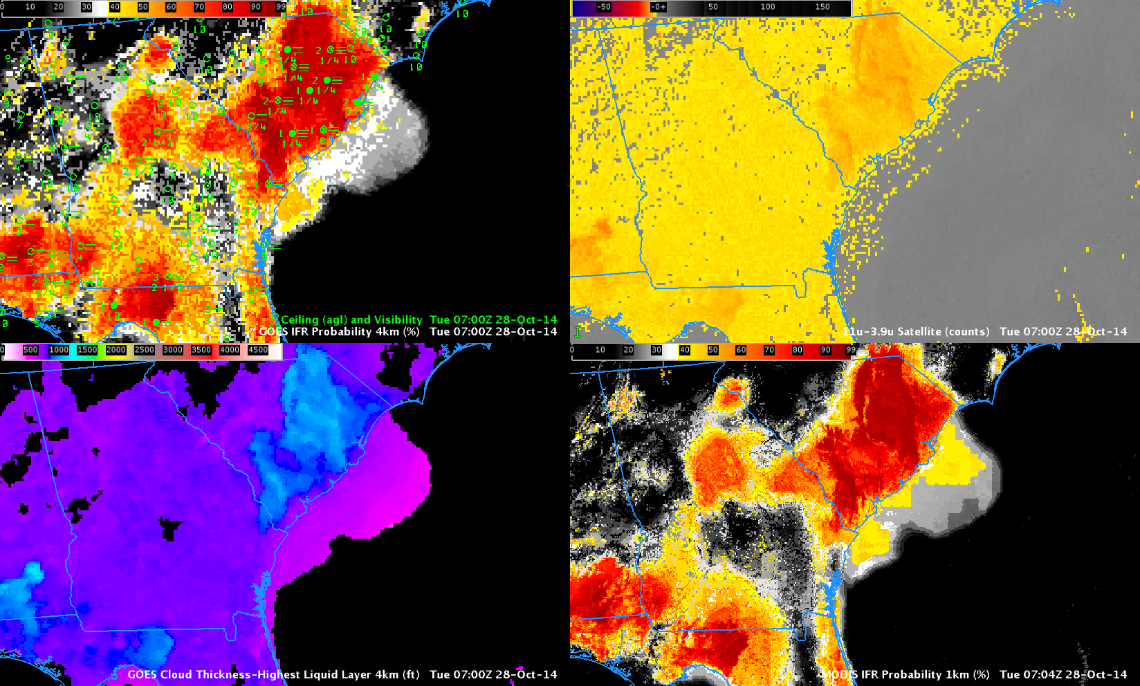
GOES-13 Water Vapor (6.5µm), Brightness Temperature Difference (10.7µm – 3.9µm) and GOES-based IFR Probabilities, all at 0615 UTC 23 October 2014, with surface observations of ceilings and visibilities (click to enlarge)

When a baroclinic system moves through a CWA, drops precipitation and then exits after sunset, the stage is often set for the development of radiation fog. The animation above cycles through the 0615 UTC imagery: GOES-13 Water Vapor (6.5 µm), GOES-13 Brightness Temperature Difference (10.7µm – 3.9µm) and GOES-based GOES-R IFR Probabilities. The upper-level reflection of a surface cold front moving through eastern Nebraska and western Iowa (link) is obvious in the (infrared) water vapor imagery, and also in the brightness temperature difference field.

The difficulty that arises with multiple cloud layers that invariably accompany these systems is that the mid- and high-level clouds do not allow for an accurate satellite-only-based depiction of low stratus and fog. GOES-R IFR Probabilities allow for that kind of depiction because near-surface saturation is considered in the computation of IFR Probabilities (using data from the Rapid Refresh Model). Thus, IFR Probabilities correctly suggest the presence of reduced visibilities over extreme northwestern Iowa and they alert a forecasters to the possibility of fog over much of western Iowa.

GOES-based IFR Probabilities, 03-13 UTC 23 October 2014 (Click to enlarge)

The animation of GOES-R IFR Probability fields, above, shows the steady increase in probability that accompanied the reduction in ceilings and visibilities. The character of the IFR Probability fields is testimony to the data that are used to create them. The fairly flat fields over Iowa early in the animation mean that satellite data cannot be used as a predictor (because of the multiple cloud levels that are present there, as apparent in the animation below). Instead, the model fields (that are fairly flat compared to satellite pixels) are used and horizontal variability in the field is small. In addition, IFR Probability values themselves are somewhat smaller because fewer predictors can be used.

IFR Probabilities are more pixelated in nature over southern Nebraska where satellite-based predictors could be used. IFR conditions are widespread in that region where IFR Probabilities exceed 90%. Note how IFR probabilities are smaller over Kansas, in a region of mid-level stratus (but not fog). The brightness temperature difference field there maintains a strong signal. IFR probability fields do a superior job of distinguishing between mid-level stratus and low stratus/fog (compared to the brightness temperature difference field). This is because a mid-level stratus deck and a fog bank can look very similar from the top, but an accurate Rapid Refresh model simulation of that atmosphere will have starkly different humidity profiles.

GOES-13 Brightness Temperature Difference (10.7µm – 3.9µm) Fields hourly from 0300 through 1300 UTC 23 October, including surface observations of ceilings and visibilities (Click to enlarge)

At 1400 UTC (below), the rising sun (and its abundant 3.9 µm energy that can be easily scattered off clouds) causes the sign of the brightness temperature difference field to flip. (Compre the 1400 UTC Brightness Temperature Difference Field below to the final Brightness Temperature Difference field (1300 UTC) in the animation above!) However, the IFR Probability field maintains its character through sunrise.

GOES-13 Brightness Temperature Difference (10.7µm – 3.9µm) and GOES-based IFR Probabilities, all at 1400 UTC 23 October 2014, with surface observations of ceilings and visibilities (click to enlarge)

The NSSL WRF accurately suggested that fog/low stratus was possible. The brightness temperature difference field from the model run, below, at 0900 UTC, shows a strong signal of low water-based clouds over western Iowa and Nebraska. (This link shows the latest model run (initialized at 0000 UTC) of Brightness Temperature Difference fields, with output from 0900 through 1200 UTC of the following day)

Simulated Brightness Temperature Difference fields, 0900 UTC 23 October 2014, from the 0000 UTC NSSL WRF Model Run (Click to enlarge)

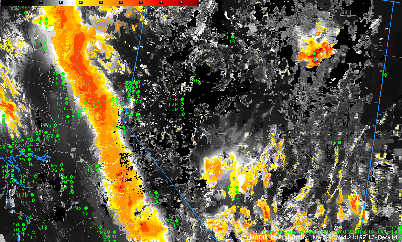
MODIS-based IFR Probability Fields were also available for this event, at 0824 UTC, below. As with the GOES, there is a noticeable (very!) difference between regions where Satellite Predictors are being used in the computation of IFR Probabilities (Nebraska) and regions where Satellite Predictors are not being used in the computation of IFR Probabilities (Iowa). The superior resolution of the MODIS data also suggests that River Valleys in eastern Nebraska are more likely foggy than adjacent land. The Elkhorn River between Norfolk and O’Neill, for example, shows up in the MODIS-based IFR Probability field as a thread of higher IFR Probability.

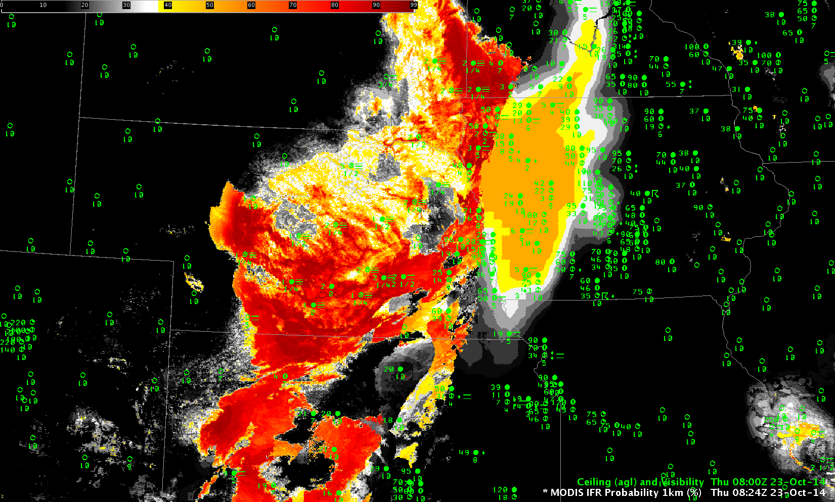
MODIS-based IFR Probability at 0824 UTC, 23 October 2014 (Click to enlarge)

GOES-R Fog Product Examples

Fog detection fusing GOES, Terra/Aqua or Suomi/NPP Satellite data with Model output