Category Archives: Day/Night Band

Stratus over Southern California

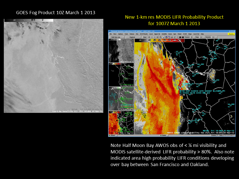
VIIRS Day/Night Band (from Suomi/NPP), GOES-R IFR Probabilities (From GOES-West) and ceilings/visibilities, all near 0900 UTC on 30 April 2013

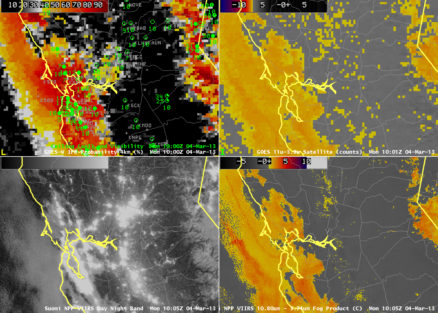
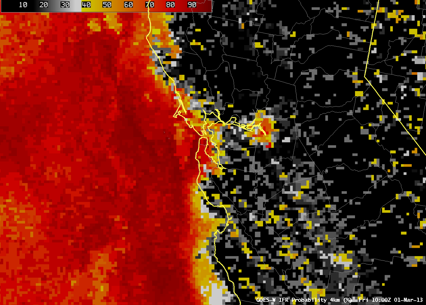
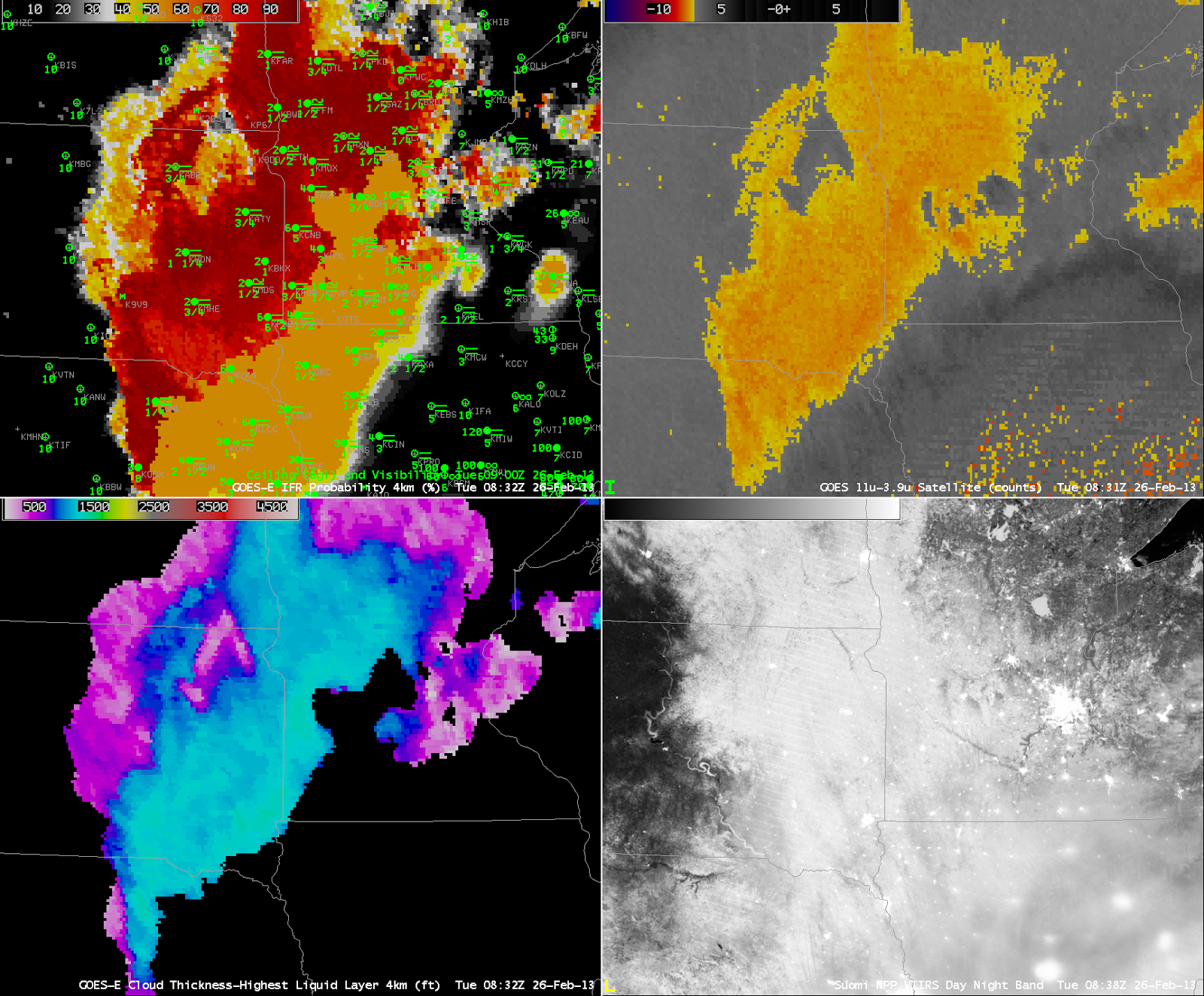
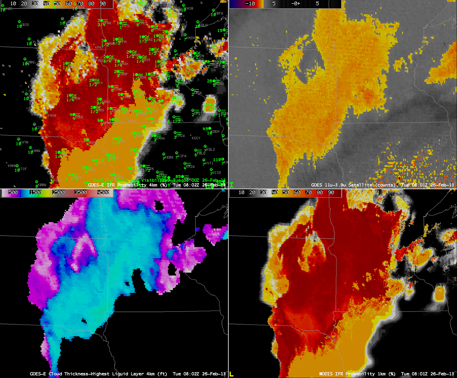
Day/Night imagery produced from VIIRS data on Suomi/NPP easily shows the large extent of marine stratus off the west coast of southern California at 0900 UTC on 30 April 2013.  That stratus may or may not be associated with low ceilings and reduced visibility that accompany IFR conditions.  A fused product that incorporates surface-based data will show where IFR conditions are most likely, and that is shown above as well.  Data from GOES-West and Rapid Refresh model output are combined to predict where IFR conditions are most likely.  Plotted observations of ceilings and visibilities confirm that the highest probabilities neatly overlay observed IFR conditions.  It is important to note that not all of the region covered by the marine stratus observed by the Day/Night band has IFR conditions.

The careful viewer may have noted that the IFR Probability fields over the ocean are quite high in regions where the Day/Night band shows no clouds at 0900 UTC.  GOES-R IFR Probabilities can be artificially enhanced in regions of Stray Light contamination in the GOES-West imager 3.7 data.  This contamination occurs around 0900 UTC at this time of year.   Note that by 1045 UTC (below), the stray light contamination has passed, and IFR probablilities over the ocean more properly align with the Day/Night band-observed cloud edges.

As above, but for 1045 UTC 30 April 2013

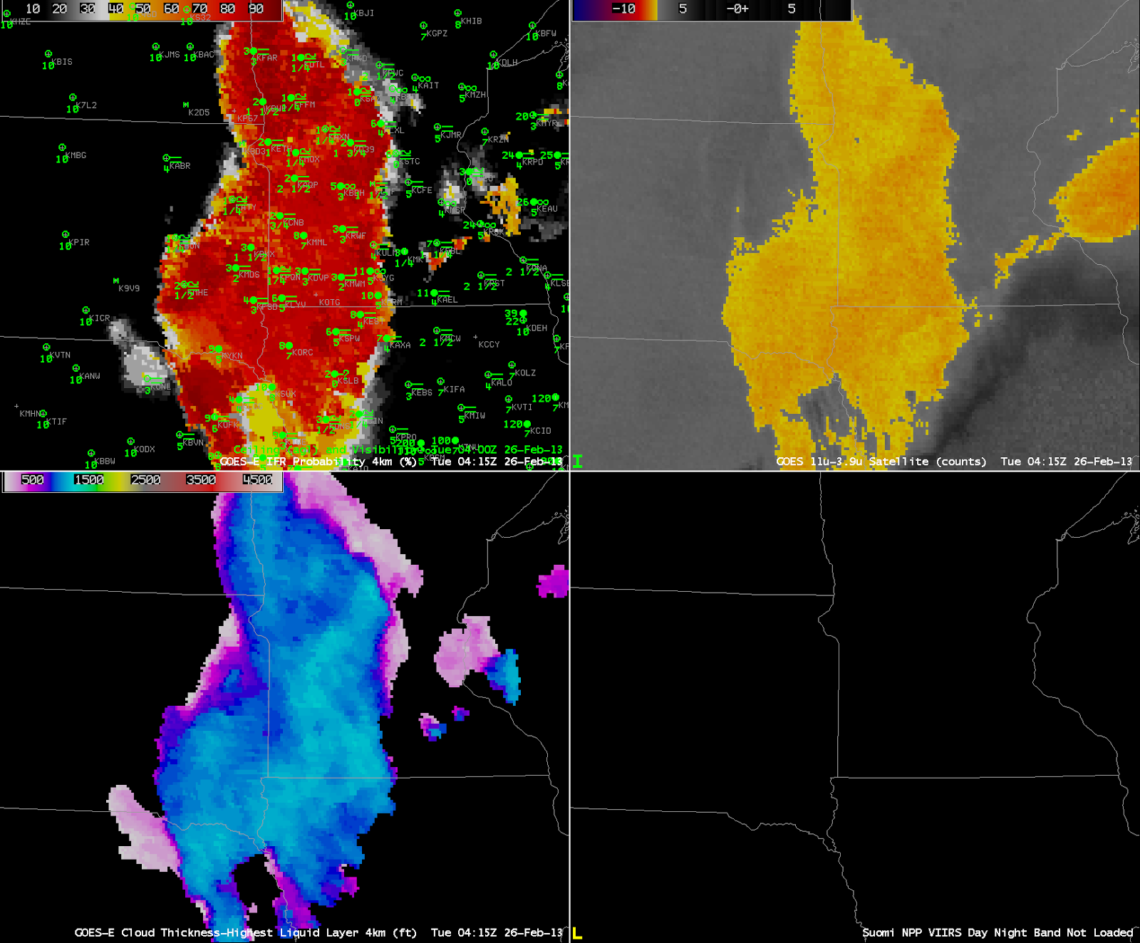
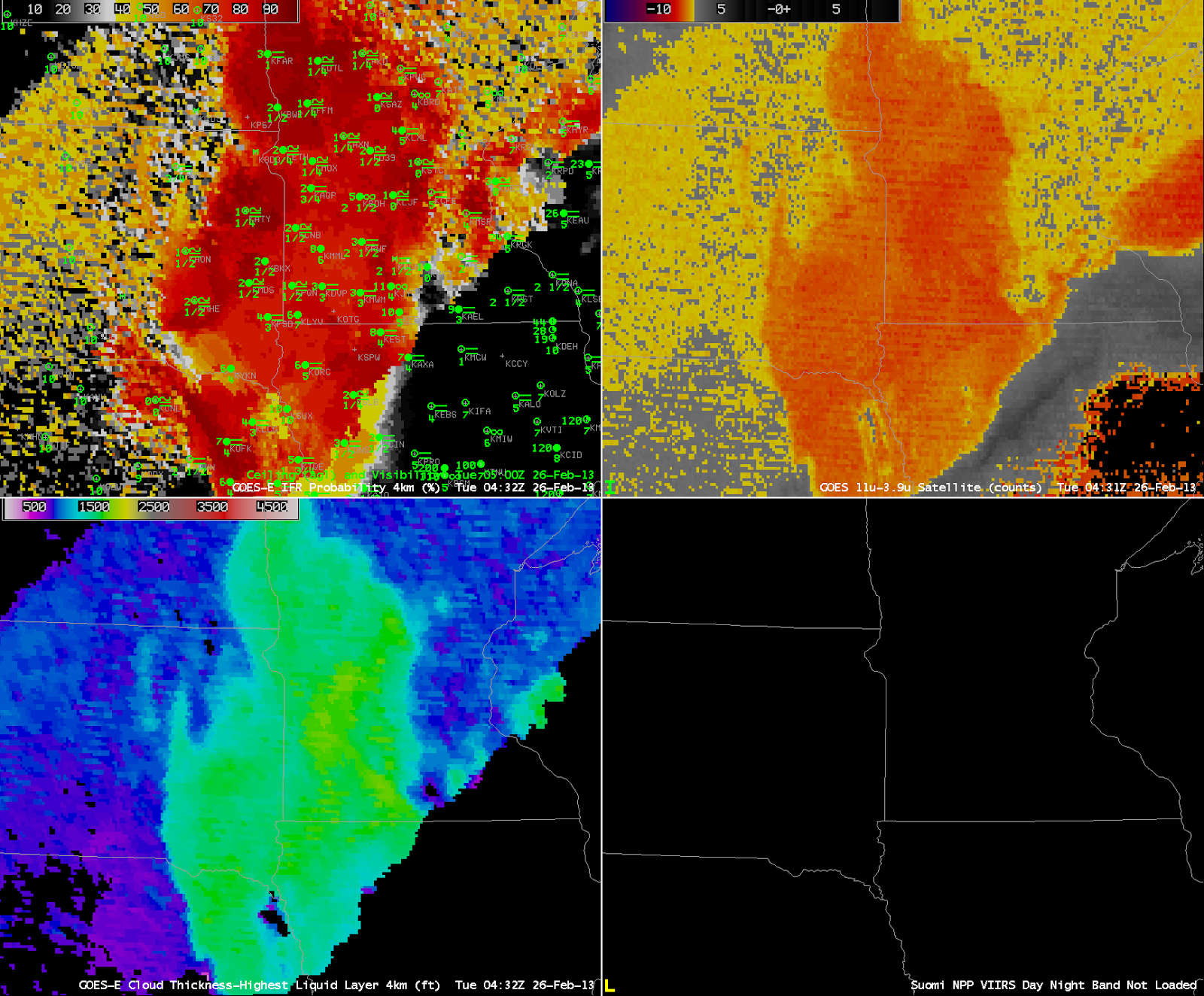
A similar set of imagery from 1045 UTC shows a general reduction in the predicted area of IFR probabilities, although the region of highest IFR probabilities, along the coast, persists and as do IFR conditions.

There was also fog over Monterey Bay on this morning.  Click here to read about it.

Radiation Fog over the Allegheny Mountains of Pennsylvania

GOES-R IFR Probabilities computed using GOES-East data, hourly from 0400 UTC through 1000 UTC (excluding 0500 UTC), 26 April 2013

GOES-R IFR Probabilities show a region over the Allegheny Mountains of northwest Pennsylvania slowly acquiring higher and higher probabilities, as ceilings and visibilities drop.  How did this product perform relative to traditional fog detection imagery (the brightness temperature difference product) and relative to data from Polar Orbiting satellites?  (The 0500 UTC imagery is excluded from the animation above because Stray Light Contamination in the 3.9 channel was apparent in the IFR probability fields).

GOES-R IFR Probability computed from GOES-East, 0332 UTC (Upper Left), GOES-East Brightness temperature Difference field (10.7µm – 3.9µm) at 0340 UTC (Upper Right), GOES-R Cloud Thickness (Lower left), GOES-R IFR Probability computed from MODIS data, 0328 UTC (Lower Left).

The ‘traditional’ method of fog detection that exploits emissivity difference of water clouds at 10.7µm and 3.9 µm, upper right in the figure above, at about 0330 UTC, just as the radiation fog was starting to develop, shows clouds detected over north-central Pennsylvania, but also from Centre County southwestward to the Laurel Highlands and to West Virginia.  GOES-based and MODIS-based IFR Probability fields have very low probabilities with these primarily mid-level clouds.

As above, but at 0615 UTC 26 April 2013

By 0615 UTC, IFR probabilities continue to increase over north-central Pennsylvania, and they remain low over southern and central Pennsylvania where mid-level clouds are reported (4100-foot ceilings at Johnstown, for example).

As above, but at 0740 UTC 26 April 2013

Another MODIS overpass at 0740 UTC better resolves the character of the developing fog and low stratus over north-central Pennsylvania.  Very high IFR probabilities in the MODIS-based fields outline the river valleys of the Allegheny Plateau in north-Central Pennsylvania.  GOES-based IFR Probabilities are high, but GOES lacks the resolution to view clearly the individual river valleys.

As above, but with Suomi/NPP brightness temperature difference (10.8 µm- 3.74µm) and Day-Night Visible imagery in the bottom right (0652 UTC), with the GOES-R IFR Probabilities (Upper Left), GOES-E Brightness Temperature Difference field (Upper Right), and GOES-R Cloud Thickness toggling between 0645 and 0702 UTC.

Suomi/NPP can also give information at high resolution about the evolving fog field.  The tendrils of fog developing in the river valleys are evident in the visible imagery created using reflected lunar illumination (A mostly full moon was present the morning of 26 April) and those water-based clouds are also highlighted in the Suomi/NPP Brightness Temperature Difference Field.  The clouds over the Laurel Highlands are higher clouds — they are casting shadows visible in the Day/Night band.

As in the figure above, but for 1015 UTC 26 April 2013

The final GOES-R Cloud Thickness field before twilight conditions, above, shows maximum thicknesses of 900 feet over Warren County, Pennsylvania, and around 850 feet over southern Clarion County.  According to this link, such a radiation fog will burn off in less than 3 hours after sunrise.  The animation below of visible imagery at 1315 and 1402 UTC shows the fog, initially widespread in river valleys at 1315 UTC mostly gone by 1402 UTC.

GOES-13 Visible Imagery, 1315 and 1402 UTC, 26 April 2013.  Warren and Clarion Counties are highlighted.

Fog over coastal North Carolina

GOES-R IFR Probabilities computed from GOES-East data, hourly from 0100 through 1200 UTC, 23 April 2013

A coastal storm along the east coast was responsible for low-level moisture over eastern North Carolina that resulted in IFR conditions.  Multiple cloud layers in the beginning of the animation above mean that IFR probabilities were computed using model data.  By 0315 UTC, however, upper level clouds had moved off the coast, leaving behind clouds at low layers that meant cloud data (brightness temperature difference) could influence the IFR probability fields;  consequently, the probability increased.  High clouds remained offshore, however, and the character of the IFR probability field shows the characteristic pixelated appearance over land — where satellite data are used in the computation of IFR probabilities — and the characteristic smoothed appearance over water where only model data are used to produce IFR probabilities.  Note how the highest IFR probabilities over eastern North Carolina do overlap the stations reporting IFR and near-IFR conditions.

GOES-R IFR Probabilities (Upper Left) computed using GOES-East, GOES-East Brightness Temperature Difference (10.7 µm- 3.9µm) (Upper Right), GOES-R IFR Probabilities computed using MODIS data (Lower Left).  All for times around 0715 UTC 23 April

The image above compares GOES-R IFR probabilities computed with MODIS and with GOES-East.  They do show very similar overall structures, with highest probabilities over land where the Brightness Temperature Difference field can contribute to the probability, and lower, smoother probability fields over water where only model data are used.  Note that both GOES-R IFR fields correctly ignore the low cloud signal over eastern South Carolina and central North Carolina.

GOES-R IFR Probabilities (Upper Left) computed using GOES-East, GOES-East Brightness Temperature Difference (10.7µm – 3.9µm) (Upper Right), Suomi/NPP Day/Night band from VIIRS (Lower Right).  Toggle for times 0615 and 0745 UTC 23 April

The GOES-based IFR probability field can also be compared to the Day/Night band sensed by VIIRS on board Suomi/NPP.  The 0609 UTC Day/Night band shows the effects of a near-full moon on the product.  The extensive cloud shield east of the Appalachians is visible, even though the image is at night, because of strong lunar illumination.  As with the traditional brightness temperature difference field, however, the cloud information from the Day/Night band gives little information about the cloud bases;  for that, the IFR probability field is needed, and low cloud bases are correctly restricted to extreme eastern North Carolina.  The Day/Night band at 0747 UTC is from a time after the moon has set;  only city lights and airglow are illuminating the clouds over Virginia and the Carolinas.  Cloud edges are still easily discerned.

Stratus and Fog over Texas

GOES-R IFR Probabilities (Upper Left) computed with GOES-East data, GOES-East Brightness Temperature Difference (10.7µm – 3.9µm) (Upper Right), Toggle between MODIS-based IFR Probabilities and Suomi-NPP Day-Night band imagery (Lower Left), Suomi-NPP Brightness Temperature Difference (Bottom Right) (10.8 µm- 3.74µm), all imagery around 0800 UTC

Stratiform clouds developed overnight in return flow from the Gulf of Mexico.  Some of the stratus was elevated, and some was closer to the surface creating IFR conditions.  The GOES imagery above captures the area of low clouds that are also visible in the Day/Night band — but the MODIS IFR Probability field suggests a difference in the stratus field near San Antonio.  Probabilities are far higher north of San Antonio’s latitude than south.  Surface observations suggest that IFR conditions are more likely where the MODIS-based IFR probabilities are highest.  (This demarcation line in the IFR Probability is far more noticeable in MODIS than in GOES).

Note that the GOES Brightness Temperature Difference field has a positive signal that is near the north-south oriented lakes in eastern Texas and western Louisiana, and that signal is absent from the VIIRS Brightness Temperature Difference field.  There is a misalignment between the 3.9 and 10.7 µm channels on GOES-13 (as discussed here) that has a maximum near 0900 UTC and that results in a false signal of low clouds.  This co-registration error can propagate into the IFR Probability field in regions where the Rapid Refresh is suggesting near-saturation at lower levels.

GOES-R IFR Probabilities (Upper Left) and surface observations of ceilings and visibility, GOES-East Brightness Temperature Difference (10.7  – 3.9) (Upper Right), Brightness Temperature at 10.7 (Lower Left) and 3.9 (Lower Right) at 1000 UTC (top image), 1215 UTC (middle image) and 1402 UTC (bottom image).

The demarcation between regions with IFR conditions and MVFR/VFR conditions becomes more distinct in the GOES-based IFR probability fields at 1000, 1200 and 1400 UTC, as shown above.  At all three times, the IFR probability field more accurately portrays the region of clouds that is most likely affecting aviation by displaying IFR conditions.

Fog/Low Stratus over San Francisco Bay

GOES-R IFR Probabilities computed from GOES-West, hourly from 0800 through 1500 UTC on 29 March 2013

The animation above shows the evolution of fog/low stratus as it moves inland from the Pacific Ocean into San Francisco Bay, and surroundings, on March 29th.  A chief forecast difficulty would be:  Will low ceilings impact San Francisco International Airport?  The TAF issued at 1212 UTC mentioned IFR conditions:

One difficulty in Fog Detection

Toggle between Suomi/NPP Day/Night Band (i.e., Night-Time Visible Imagery, 0.70 µm) and Brightness Temperature Difference field (10.8 µm- 3.74 µm) at 0734 UTC on 28 March 2013

The image toggle above shows an area of stratus over central Missouri and surrounding states.  The stratus shows up in both the Night-time visible Day/Night band from Suomi/NPP (March 28th is one day past the Full Moon, so there is plenty of lunar illumination, and indeed lunar shadows from the higher cirrus clouds over Illinois, Kentucky and Tennessee are apparent).  The brightness temperature difference field crisply highlights the region of lower, water-based clouds.  That difference field arises from the differences in emissivity properties of the water-based clouds:  they emit nearly as a blackbody around 11 µm, and not as a blackbody at 3.9 µm.

A key question for this scene is:  is this cloud that is depicted stratus at mid-levels, or is it fog?  From the top (that is, as the satellite views it), a stratus deck will look very much like a fog bank.  The satellite gives little information, however, on how thick the cloud is, or on how close to the ground it sits.  A satellite-only fog detection algorithm, therefore, will include many false positives.

MODIS-based IFR probabilities, 0811 UTC on 28 March 2013

IFR probabilities include data about the surface that are incorporated into the Rapid Refresh Model.   This fused product clarifies where the brightness temperature difference product is detecting mid-level stratus versus low-level fog.  In this case over Missouri, IFR probabilities are very low throughout the scene because saturation at low levels in the Rapid Refresh is not occurring, and therefore IFR probabilities are low.

By blending information about the top of the cloud (the brightness temperature difference product) with information about the bottom of the cloud (the Rapid Refresh model data), a more accurate depiction of the horizontal extent of IFR conditions is achieved.

Cold frontal passage in Oregon

GOES-R IFR Probabilities (Upper Left), GOES-West Brightness Temperature Difference (10.7 µm – 3.9 µm) (Upper Right), Topography (Lower Left), GOES-West Water Vapor Imagery (6.7 µm) (Lower Left), hourly from 0400 through 1700 UTC 20 March 2013.

The animation above of the Fog/Low Stratus and Brightness Temperature difference highlights the difficulty that the traditional brightness temperature difference product encounters when multiple cloud layers are present, as you might expect to be present given the water vapor imagery.  At the beginning of the animation, highest IFR probabilities exist over the elevated terrain that surrounds the Willamette Valley in Oregon.  There were also high probabilities off shore.  As the frontal region moves onshore, IFR probabilities increase on shore.   Note also how the GOES-R IFR Probability field is a more coherent one whereas the traditional brightness temperature difference field from GOES contains many separate areas of return that make it harder to see the big picture.  The brightness temperature difference also suffers from stray light contamination at 1000 UTC — but that contamination does not propagate into the GOES-R IFR probability field.

GOES-R IFR Probabilities computed from GOES-West (Upper Left), GOES-West Brightness Temperature Difference (10.7 µm – 3.9 µm) (Upper Right), Topography (Lower Left), Toggle between Suomi/NPP Brightness Temperature Difference (10.8 µm – 3.74 µm) and Day/Night Band, all imagery near 1000 UTC on 20 March 2013

The imagery above shows how straylight contamination in the shortwave IR (3.9 µm) can influence the brightness temperature difference.  The GOES imagery shows the effects (just at this 1000 UTC image, which is also included in the animation above), but that ‘contamination’ does not propagate strongly into the GOES-R IFR Probability.  Note also that the Suomi/NPP Brightness Temperature Difference shows none of the stray light contamination.  Lunar illumination  allows the nighttime visualization of the clouds off the west coast of the US.  As this frontal band moves over Oregon, reduced visibilities result, but only the GOES-R IFR probabilities accurately capture the location of the frontal band because of the multiple cloud layers that exist.

Fog near San Francisco

GOES-R IFR Probabilities computed from GOES-West (Upper Left), GOES-West Brightness Temperature Difference (10.7 µm – 3.9 µm) (Upper Right), Suomi/NPP VIIRS Day/Night Band (Lower Left), Suomi/NPP VIIRS Brightness Temperature Difference (10.8 µm- 3.74 µm) (Lower Right), all images near 1000 UTC on March 4 2013.

A high-impact fog event on March 1st led to a Group Stop at SFO International.  The synoptic conditions that supported fog development on 1 March (Images from 1 March are shown at the bottom of this blog post) persisted through the weekend along the West Coast, and fog was again observed on Monday morning, 4 March and the four images above show results from fog detection schemes for that date.  The GOES-R Fog/Low Stratus IFR Probability field shows that the highest probability of IFR conditions is occurring where IFR and near-IFR conditions are observed.  Note the benefits of the high-resolution Suomi/NPP VIIRS data.  Sharp edges to the low cloud field are ably captured in central Santa Clara County.  There are also benefits to using the near infrared and infrared channels to detect regions of low clouds in urban areas, where bright lights can dazzle the Day/Night band so that small breaks in the clouds, as detected just south and west of southern San Francisco Bay, cannot be discerned in the visible.  Compare the differences in the 1-km data from VIIRS to the nominal 4-km resolution of present GOES in the imagery above.  Note also that the brightness temperature difference helps distinguish between snow and clouds over the Sierra Nevada.

GOES-R IFR Probabilities computed from GOES-West, hourly, from 0400 UTC to 1600 UTC on 4 March 2013

The animation, above, of GOES-R IFR Probabilities helps describe and define the region of evolving IFR conditions early on March 4th.

Figures provided by Warren Blier, WFO MTR.

Warren Blier from NWS in MTR sent along an email about the event on March 1st.  The screen capture above shows MODIS-based GOES-R IFR probabilities (on the right) compared with the GOES-West ‘traditional’ unenhanced  brightness temperature difference.  The higher spatial resolution of MODIS and of VIIRS really does pick up the details.  The image below is the 1000 UTC image created using GOES-West data, and the comparison between the MODIS image above and the GOES image below shows the power of MODIS resolution.

GOES-R IFR Probabilities computed using GOES-West data, 1000 UTC on 1 March 2013

An animation of GOES-R IFR probabilities from 0000 through 1600 UTC on 1 March shows the highest IFR probabilities increasing near SFO after 0900/1000 UTC on the first.

Hourly imagery of IFR probabilities computed from GOES-West, 0000 through 1600 UTC on March 1st

IFR conditions in Maine

GOES-R IFR Probabilities computed from GOES-East (Upper Left), GOES-East Brightness Temperature Difference (10.7 µm – 3.9 µm) (Upper Right), GOES-R Cloud Thickness (Lower Left), Toggle between Suomi/NPP Brightness Temperature Difference (10.8 µm – 3.74 µm) and Day/Night Band “Nighttime Visible” imagery (Lower Right), all around 0815 UTC on 28 February

Weak Low pressure in the Gulf of Maine helped generate IFR conditions over the northeastern United States early in the morning on 28 February 2013.  The brightness temperature difference fields over New England from Suomi/NPP include very sharp cloud edges (also present in the Day/Night band imagery).  Because the GOES-R IFR Probability field also includes information from the Rapid Refresh, it is better able to distinguish fog and low stratus, as present over most of Maine, from elevated stratus, present over western New Hampshire and Quebec.

GOES-R IFR Probabilities computed from GOES-East (Upper Left), GOES-East Brightness Temperature Difference (10.7 µm – 3.9 µm) (Upper Right), GOES-R Cloud Thickness (Lower Left), Suomi/NPP Brightness Temperature Difference (10.8 µm – 3.74 µm) (Lower Right), times as indicated

The animation of the imagery, above, demonstrates how the GOES-R IFR probability product can be used to monitor the evolving nature of a low cloud field.  As the low pressure system in the Northeast starts to move away, the fog/low clouds rotate eastward.   Two noteworthy events in the loop are present.  The 0515 UTC imagery (mislabeled as 0510 UTC), contains stray light in the 3.9 µm field, and the traditional GOES brightness temperature difference field is therefore changed significantly, but the GOES-R IFR probability field is not.  Note also that multiple cloud layers exist over coastal Maine and New Hampshire at the end of the animation, but GOES-R IFR probabilities correctly maintain high probabilities in a region where IFR conditions are present and where the traditional brightness temperature difference field does not show a signal consistent with low clouds.

IFR conditions over the upper Midwest

GOES-R IFR Probabilities from GOES-East (Upper Left) at 0832 UTC, along with 0900 UTC observations, Traditional GOES-East Brightness Temperature Difference (10.7  µm – 3.9  µm) at 0832 UTC (Upper Right), GOES-R Cloud Thickness computed from GOES-East (Lower Left), Suomi/NPP Day/Night Band Nighttime visible imagery, 0838 UTC (Lower Left)

Stratus and low clouds persisted over western Minnesota and the eastern Dakotas overnight on 25 to 26 February, and the GOES-R IFR Probability field ably captured the region of lowest visibility.  Note that the IFR probability field extends into northwest Iowa (albeit with relatively lower probabilities).  This is a region where high-level cirrus prevents the traditional brightness temperature difference product from giving useful information about the low levels.  In this region, Rapid Refresh data are used to fill in information and more accurately capture the region of IFR conditions.

As above, but for 0802 UTC for GOES-East Products, and with the MODIS-based IFR probability field at 0801 UTC in the lower left

GOES-R IFR Probabilities can be used with MODIS data as well, and the better resolution (1 km at nadir vs. 4 km at GOES nadir) means the MODIS fields have better small-scale detail.    Note, for exanple, the sharper edge to the IFR probability field in east-central Minnesota.

As at the beginning of the post, except for 0415 UTC (top), 0432 UTC (middle) and 0445 UTC(bottom)

Stray-light issues can influence the 3.9 µm imagery, and therefore the brightness temperature difference field, and therefore the GOES-R IFR Probability field.  In the three images above, Stray Light is noteable in the 3.9 µm at 0432 UTC, but that erroneous information can be de-emphasized in the GOES-R IFR probability field because the Rapid Refresh Data in regions where Stray Light is present may show dryer low levels.