Category Archives: Day/Night Band

IFR Conditions over Oklahoma and Kansas

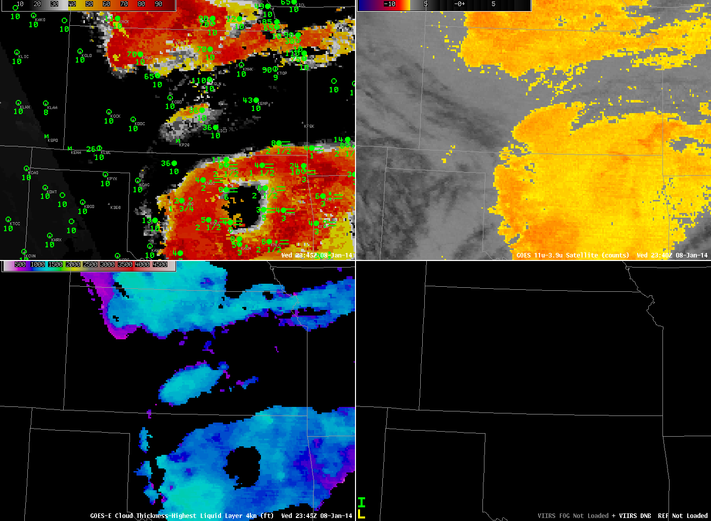
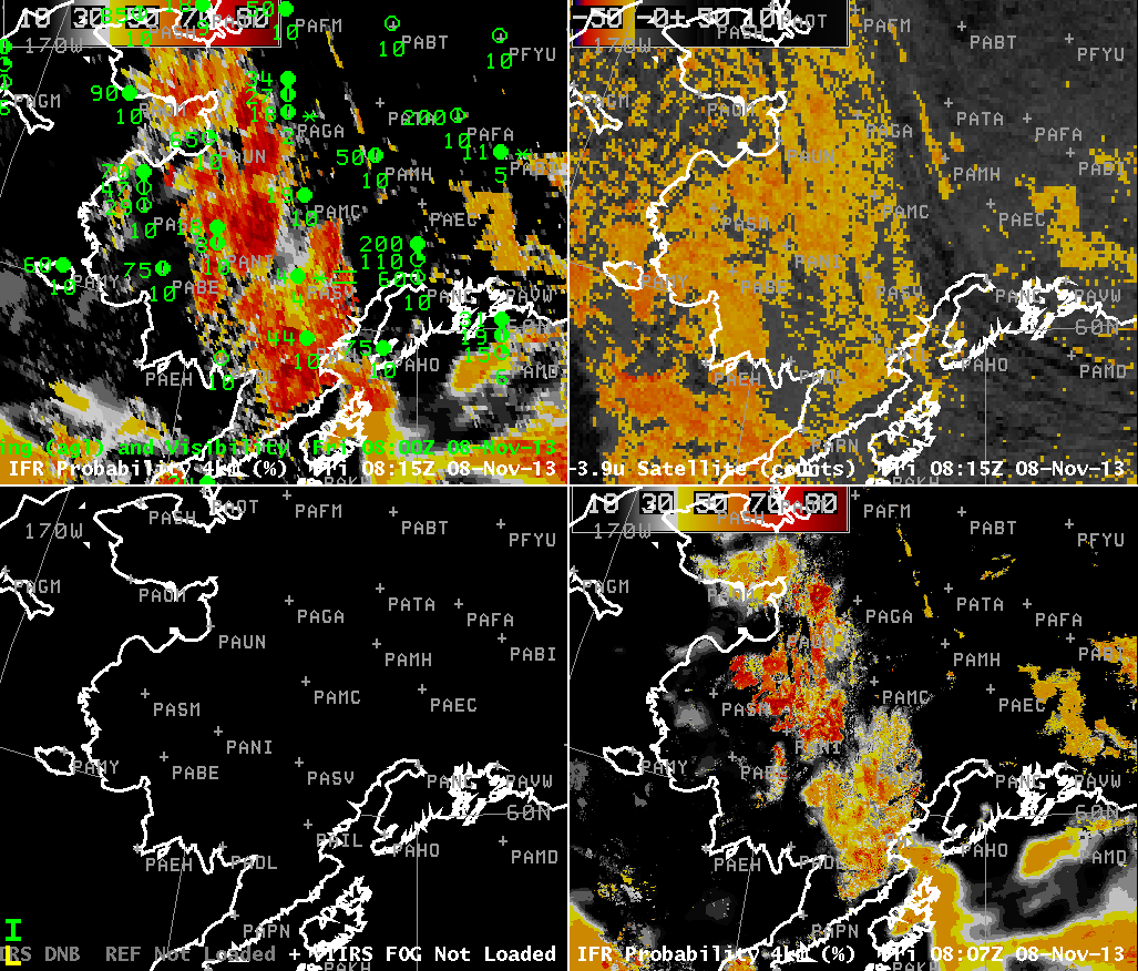
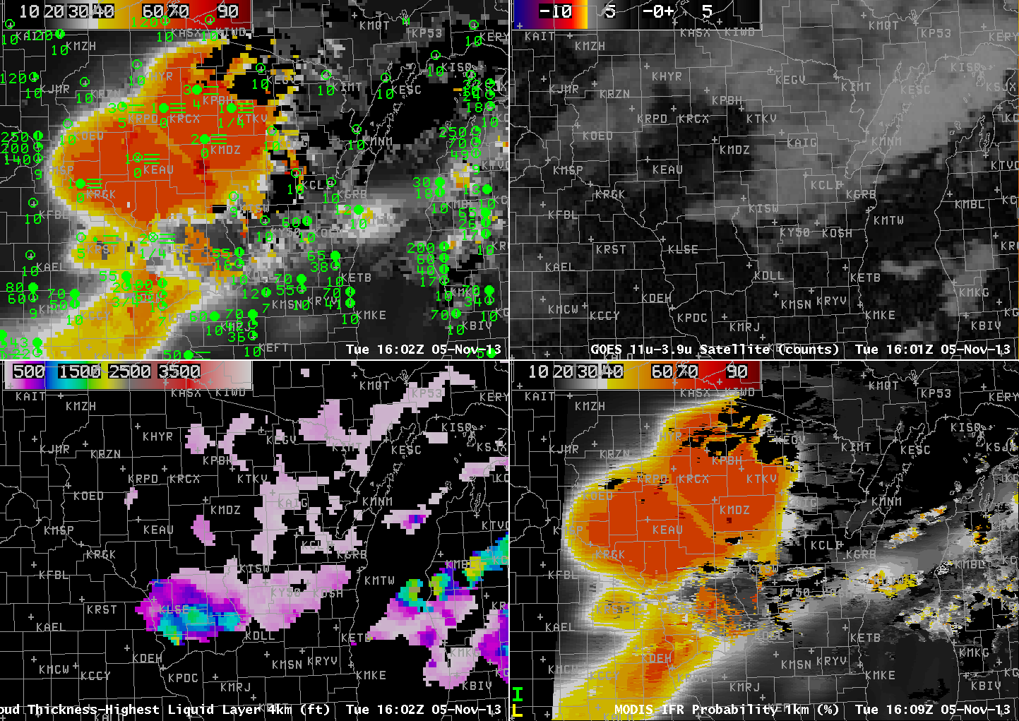
GOES-R IFR Probabilities from GOES-13 (upper left), GOES-13 Brightness Temperature Difference (10.7 µm – 3.9 µm) Fields (upper right), GOES-R Cloud Thickness from GOES-13 (lower left), Suomi/NPP Day/Night Band (lower right), ~2345 UTC 8 January 2014 (click image to enlarge)

IFR Conditions developed over portions of Kansas and Oklahoma (and adjacent states) overnight. How did the GOES-R IFR Probability field diagnose the development of this event? At ~0000 UTC, the traditional method of low stratus/fog detection (Brightness Temperature Difference) showed two regions over the Plains, one centered over Oklahoma, and one over the Kansas/Nebraska border. IFR Probabilities at the same time covered a smaller area; Wichita in particular had low IFR Probabilities despite a brightness temperature difference signal, and Wichita did not report IFR conditions at the time.

Note that high clouds are also present in the Brightness Temperature Difference field over western Kansas, the panhandles of Texas and Oklahoma, and New Mexico. In the enhancement used, high clouds are depicted as dark greys.

As above, but at 0202 UTC 9 January 2014 (click image to enlarge)

By 0200 UTC (above), the high clouds have moved over parts of Oklahoma and Kansas. Consequently, there are regions over central Oklahoma and south-central Kansas where the brightness temperature difference field is not useful in detecting low stratus/fog that is occurring. The IFR Probability fields suggest the presence of low clouds despite the lack of satellite data because the IFR Probability Field also uses output from the Rapid Refresh Model that suggests saturation is occurring in those regions. Model data are also used where satellite data suggest low clouds/stratus are present to delineate where surface ceilings/visibilities are congruent with IFR conditions. As at 2345 UTC, Wichita is not reporting IFR conditions, although the brightness temperature difference field suggests IFR conditions might exist. The IFR Probability field correctly shows low values there.

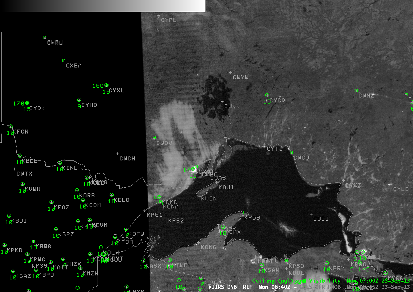
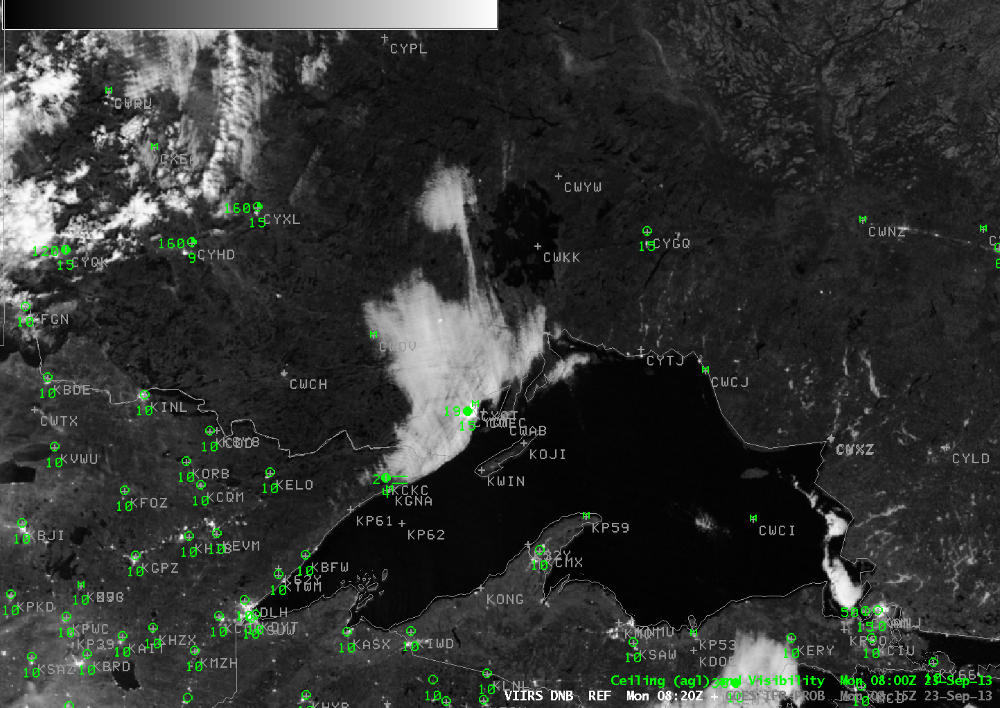
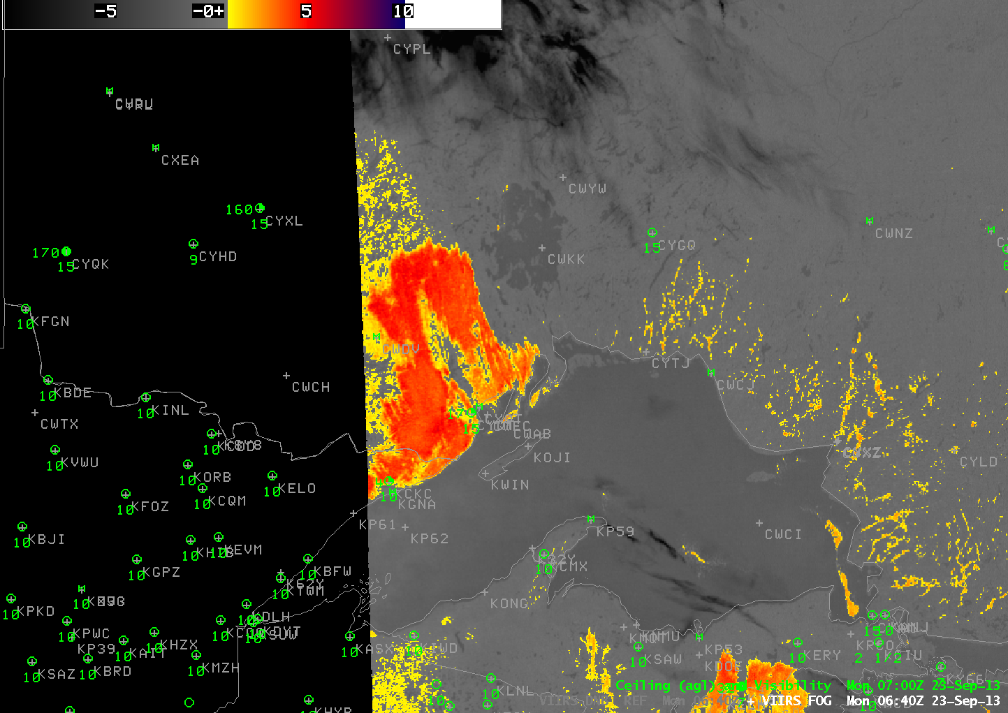
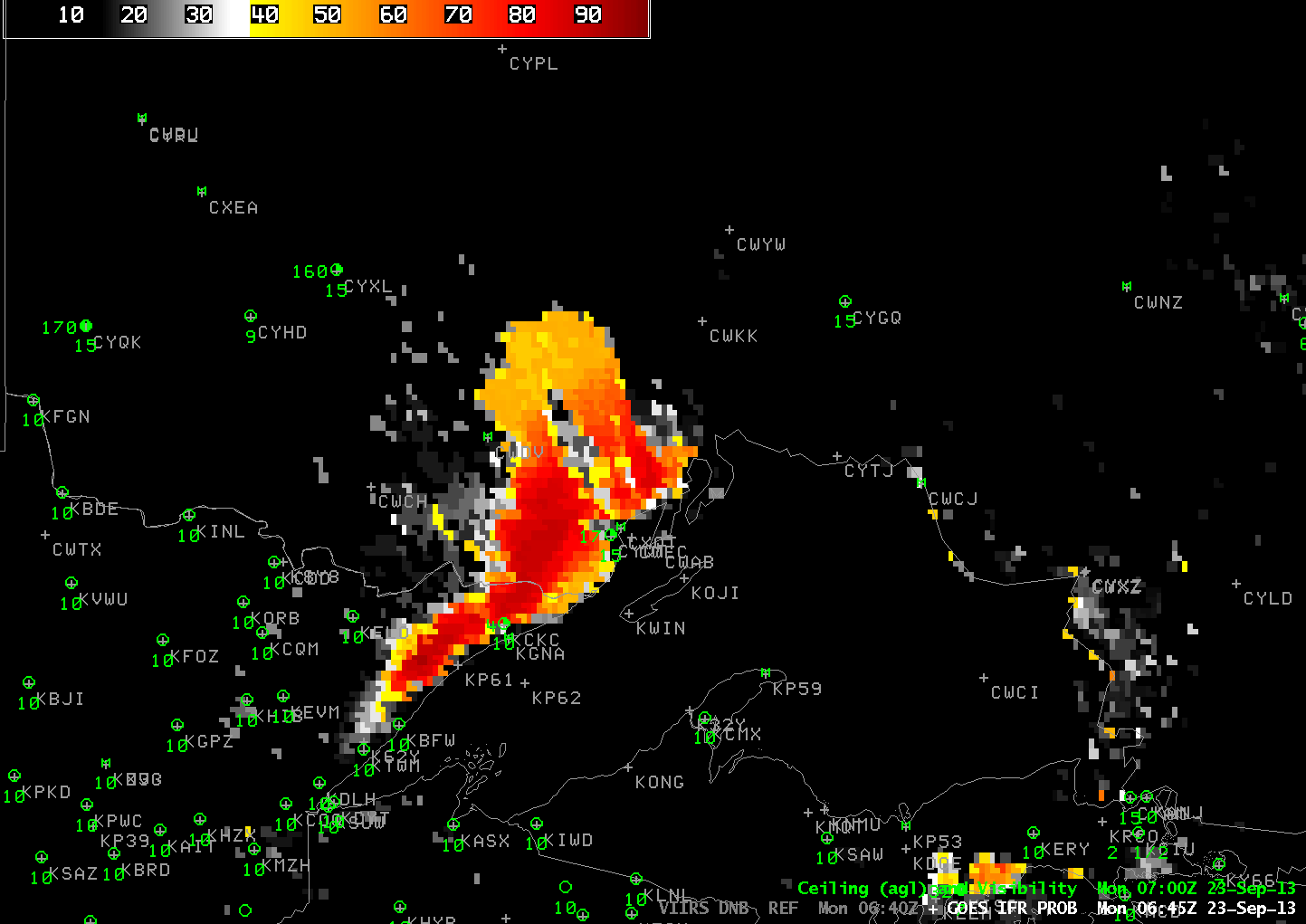
As above, but at 0802 UTC 9 January 2014. Suomi/NPP data is a toggle of Day/Night band and 11.35 µm – 3.74 µm brightness temperature difference (click image to enlarge)

By 0802 UTC, high clouds have overspread much of Oklahoma, yet IFR conditions are occurring at several locations. IFR probabilities nicely depict the widespread nature of this IFR event. Probabilities are reduced in regions where high clouds are present because the algorithm cannot use satellite predictors of low clouds/stratus there. Both the Day/Night band and the brightness temperature difference field give information about the top of the cloud deck — it’s hard to infer how the cloud base is behaving. The addition of Rapid Refresh model information on low-level saturation helps better define where IFR conditions are present.

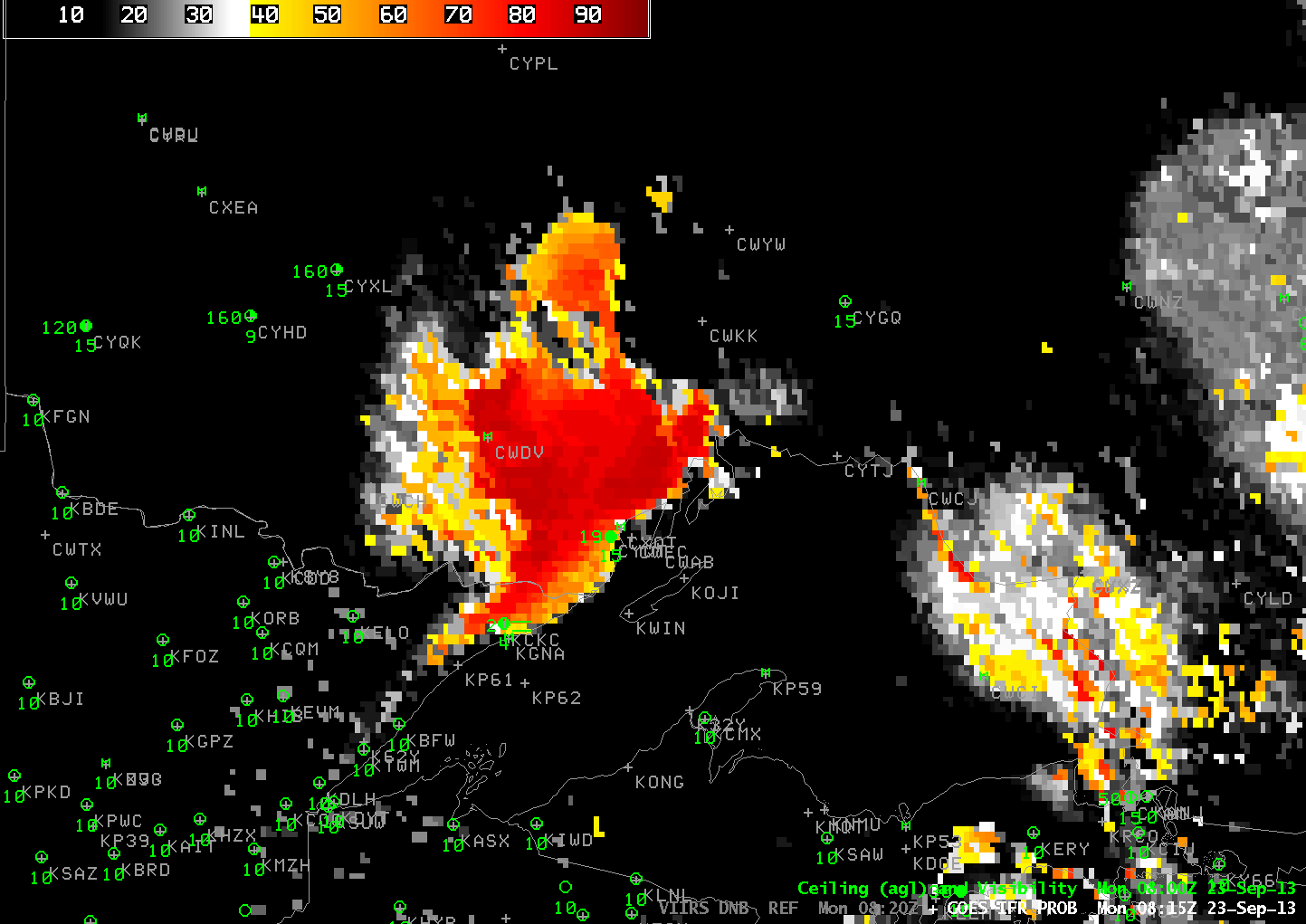
As above, but at 0945 UTC 9 January 2014. Suomi/NPP data is a toggle of Day/Night band and 11.35 µm – 3.74 µm brightness temperature difference (click image to enlarge)

By 0945 UTC, above, the time of the next Suomi/NPP overpass, the high clouds have started to move eastward out of Oklahoma. Consequently, satellite data can be used as one of the predictors in the IFR probability field, and IFR Probabilities over Oklahoma increase. By 1215 UTC (below), higher clouds have east out of the domain, and IFR Probabilities are high over the region of reduced ceilings/visibilities over Oklahoma. The algorithm continues to show lower probabilities in regions over Kansas where the Brightness temperature difference signals the presence of low stratus/fog but where IFR conditions are not present. Again, this is because the Rapid Refresh model in those regions is not showing low-level saturation.

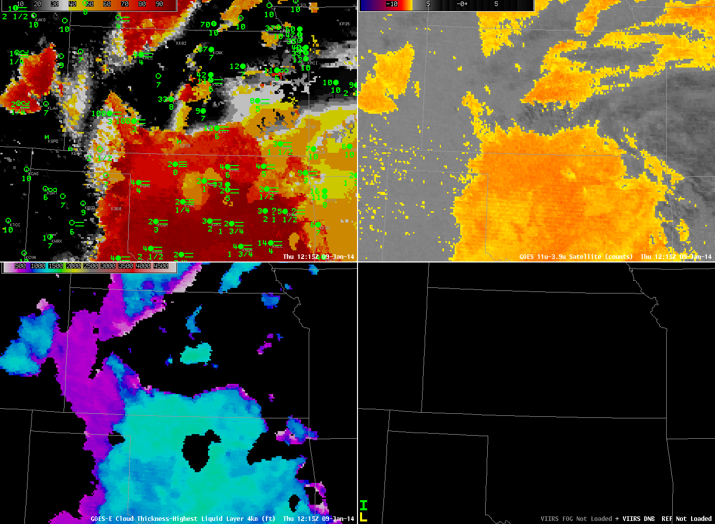
As above, but at 1215 UTC 9 January 2014 (click image to enlarge)

Note in the imagery above how the presence of high clouds affects the GOES-R Cloud Thickness. If the highest cloud detected is ice-based, no cloud thickness field is computed. GOES-R Cloud Thickness is the estimated thickness of the highest water-based cloud detected. If ice clouds are present, the highest water-based cloud cannot be detected by the satellite. Cloud Thickness is also not computed during twilight conditions. Those occurred just before the first image, top, and about an hour after the last image, above.

IFR Probabilities over the Pacific Northwest with a front

GOES-R IFR Probabilities from GOES-15 (upper left), GOES-15 Brightness Temperature Difference (10.7 µm – 3.9 µm) Fields (upper right), GOES-R Cloud Thickness from GOES-15 (lower left), Suomi/NPP Brightness Temperature Difference (lower right), times as indicated, 3 January 2014 (click image to animate)

One benefit of the GOES-R IFR probabilities is its consistency from hour to hour. In the animation above, the region of higher IFR Probabilities associated with a southward-propagating front over Oregon shows good hour-to-hour consistency. In contrast, the Brightness Temperature Difference field (upper right in the figure) suffers from the presence of higher clouds (denoted in the enhancement by darker regions). As the high IFR Probabilities expand southward into southern Oregon, reported visibilities/ceilings decrease towards IFR conditions. In the animation, regions of high clouds show up in the Cloud Thickness product as regions of missing data: Cloud Thickness is of the highest water-based cloud. If the highest cloud detected by satellite is mixed-phase, or ice, Cloud Thickness is not computed. Cloud Thickness is also not computed in the 1600 UTC imagery because that time is near sunrise, and cloud thickness is not computed in twilight conditions.

Suomi/NPP provided a view of the scene as well, and the Day/Night Band showed the band of frontal clouds well. The brightness temperature difference field suggests that the cloud band was not necessarily low cloudiness, although the higher IFR Probabilities (and reduced ceilings and visibilities) testify to the presence of low clouds underneath the middle- and higher-level clouds.

GOES-R IFR Probabilities from GOES-15 (upper left), GOES-15 Brightness Temperature Difference (10.7 µm – 3.9 µm) Fields (upper right), GOES-R Cloud Thickness from GOES-15 (lower left), Toggle between Suomi/NPP Day/Night band and Brightness Temperature Difference (lower right), ~1000 UTC, 3 January 2014 (click image to enlarge)

Fog over snow in the upper midwest

Suomi/NPP Brightness Temperature Difference (11.35 µm – 3.74 µm) Brightness Temperature Difference and Day/Night Band, 0840 UTC 27 December 2013 (click image to enlarge)

At times of low lunar illumination, it can become increasingly difficult to discern regions of clouds and snow in the Suomi/NPP day/night band, shown above, toggling with the brightness temperature difference. Nevertheless, careful perusal of the image reveals cloud edges over northeastern Wisconsin and through central lower Michigan that are confirmed by the brightness temperature difference field. In contrast, the whiter region that stretches southwestward from Des Moines towards extreme northeastern Kansas has no signal in the brightness temperature difference field. This is snow on the ground (vs. little snow to the northwest).

GOES IFR Probabilities computed with GOES-13 data, hourly from 0615 UTC through 1302 UTC, 27 December 2013 (click image to enlarge)

IFR Probability fields and GOES-Based brightness temperature difference fields are produced to aid in the detection of low clouds. In the animation above, higher IFR probabilities are centered on north-central Wisconsin where, intially, IFR conditions are not quite met (according to the plotted observations of ceiling and visibilities). However, as the night progresses, ceilings lower and visibilities decrease as IFR conditions do develop in regions where IFR Probabilities are high. The IFR probabilities roughly overlap the region where IFR conditions exist.

Note that encroachment of higher clouds in from the west, starting around 0800 UTC, means that satellite data cannot be used in the IFR Probability algorithm. Because only model data are used, IFR probabilities drop from values at/above 80% to values between 50 and 60% even as IFR conditions come to be more widespread. For this reason, it is important when interpreting IFR Probabilities to be alert to the presence of high clouds.

IFR Probabilities give a much more better approximation of where fog/low stratus may be occurring than a simple brightness temperature difference field. The toggle between the GOES-R IFR Probabilities and the GOES-13 Brightness Temperature Difference, below, gives testimony to this.

Fog/Low Stratus over southwest Alaska on November 8

GOES-15-based GOES-R IFR Probabilities every half hour from 0300 UTC through 1530 UTC (click image to animate)

Fog and low stratus were present over southwestern Alaska early on November 8. How did the GOES-R IFR Probability fields perform compared to the heritage brightness temperature difference (in this case, 10.7 µm – 3.9 µm from GOES-15). Consider the airport PARS (southwest of Anvik — PANV and northwest of Aniak — PANI). IFR conditions are present there until 0900 UTC, when ceilings rise and IFR probabilities drop. Subsequently, IFR Probabilities increase again as a north-south oriented region of higher IFR probabilities moves over, and IFR conditions are again present by 1600 UTC. Further south, PAJZ and PAIG report IFR conditions when IFR Probabilities are high, and conditions improve as IFR Probabilities decrease. IFR Probabilities initially around PAIG have the characteristic flat field (and somewhat lower probability) associated with a region where high-level clouds are present. In these regions, only Rapid Refresh data can be used to compute the probability; because satellite predictors are not used, the computed IFR probabilities are lower.

Compare the IFR Probability field, above, to the Brightness Temperature Difference field, below, that has been color-enhanced to highlight regions where water-based clouds may be present. The IFR Probability field correctly reduces the regions where IFR conditions might be occurring. That is, the traditional brightness temperature difference field is plagued by many false positives. This is because mid-level stratus that is unimportant for transportation looks to a satellite to be very similar to low-level stratus that is important for transportation.

GOES-15 Brightness Temperature Difference (10.7 µm – 3.9 µm) every hour from 0300 UTC through 1500 UTC (click image to animate)

MODIS data from the polar-orbiting satellites Terra and Aqua can also be used to compute IFR Probabilities, and MODIS data — although less frequent than the data from the geostationary GOES-15 — has far superior horizontal resolution (nominal MODIS resolution is 1 km at nadir) to GOES data (nominally 4 km at the sub-satellite point over the Equator) over Alaska. Small-scale features are much more likely to be detected in MODIS data, as shown below.

GOES-15-based GOES-R IFR Probabilities (Upper Left), GOES-15 Brightness Temperature Difference Product (10.7 µm – 3.9 µm) (Upper Right), Suomi-NPP Brightness Temperature Difference (11.45 µm – 3.74 µm) and Day/Night band (Lower Left), MODIS-based GOES-R IFR Probabilities (Lower Right), all times as indicated (click image to enlarge)

The Day/Night band from Suomi/NPP can sometimes be used to detect cloud features. However, when the Moon is not present to provide illumination, cloud detection is a challenge. In the toggle above between the Day/Night band and the brightness temperature difference from VIIRS (11.45 – 3.74), for example, there is little evidence of the apparent cloud edge that is visible both in VIIRS data, in GOES-15 data (Upper right) and in the IFR Probability fields from GOES (Upper Left) and MODIS (Lower Right).

Fog and Stratus in one scene: What should be highlighted?

GOES-13-based GOES-R IFR Probabilities (Upper Left), GOES-13 Brightness Temperature Difference Product (10.7 µm – 3.9 µm) (Upper Right), GOES-R Cloud Thickness (Lower Left), Suomi-NPP Day/Night band (Lower Right), all times as indicated (click image to enlarge)

Dense fog developed over Western Wisconsin before sunrise on 5 November 2013. The animation above shows the development of high IFR probabilities in that region as a mid-level stratus deck shifts off to the east. Cloud thicknesses just before sunrise reach 1100 feet over portions of Wisconsin; according to this plot, fog should persist for at least 4 hours after sunrise. This was the case. Fog dissipated shortly after 1700 UTC.

This case shows a benefit of the GOES-R IFR Probability field: it accurately discerns the difference between low stratus/fog (that develops over western Wisconsin) and mid-level stratus (retreating to the east over central and eastern Wisconsin during the animation). Mid-level stratus is normally not a transportation concern whereas low clouds/fog most definitely are; in this case, dense fog advisories were issued by the Lacrosse, WI, WFO (ARX). At the beginning of the animation, widespread mid-level stratus is indicated (IFR conditions are not reported). As the night progresses, IFR Probabilities increase in regions where IFR conditions start to be reported. (A brightness temperature signal in GOES also develops in this region).

As above, but at 0815 UTC. The lower right image toggles between the Day/Night Band and the Brightness Temperature Difference (11.45 µm – 3.74 µm) from Suomi/NPP (click image to enlarge)

Suomi/NPP VIIRS viewed this scene shortly after 0815 UTC, and that imagery is above. Both the Day/Night band and the Brightness Temperature Difference fields (11.45 µm – 3.74 µm) are shown as a toggle. The mid-level stratus at 0815 is readily apparent. The developing fog over river valleys in western Wisconsin shows plainly in the brightness temperature difference field, but less so in the day/night band with scant lunar illumination.

GOES-13-based GOES-R IFR Probabilities (Upper Left), GOES-13 Brightness Temperature Difference Product (10.7 µm – 3.9 µm) (Upper Right), GOES-R Cloud Thickness (Lower Left), MODIS-based IFR Probabilities (Lower Right), all times as indicated (click image to animate)

MODIS data from Terra and Aqua is also used to produce IFR Probabilities, and those data are shown above, for three times: 0413 UTC, 0823 UTC and 1609 UTC. Patterns in the MODIS IFR Probability are similar to those in GOES, but small-scale features such as river valleys are much more apparent. Note that by 1609 UTC, higher clouds have overspread western Wisconsin in advance of an approaching mid-latitude cyclone; thus, the GOES and MODIS IFR Probabilities both are flat fields that are mostly based on Rapid Refresh data. Nevertheless, they both depict the region of IFR conditions over western Wisconsin that is surrounded by better visibilities and higher ceilings. Recall that GOES-R cloud thickness is not computed where high clouds are present.

Fog and Stratus under high clouds in the Southern Plains

GOES-13-based GOES-R IFR Probabilities (Upper Left), GOES-13 Brightness Temperature Difference Product (10.7 µm – 3.9 µm) (Upper Right), MODIS-based GOES-R IFR Probabilities (Lower Left), Suomi-NPP Brightness Temperature Difference (11.35 µm – 3.74 µm) and Day/Night band (Lower Right), all times as indicated (click image to enlarge)

Fog and low stratus developed over the Southern Plains during the morning hours of 28 October 2013. The imagery above, from near 0730 UTC, demonstrates strengths of the IFR Probability fields and inherent limitations to the traditional methods of detecting fog and low stratus: the brightness temperature difference between 10.7 µm and 3.9 µm data. For example, note the elevated stratus over the Red River Valley in southeastern OK. Both GOES and VIIRS Brightness Temperature Difference fields there show a strong signal (and the day/night band also suggest clouds are present); IFR Probabilities are low, however, and are in good agreement with the observed ceilings and visibilities that show MVFR conditions.

The brightness temperature difference fields from both Suomi/NPP and from GOES show high clouds over south-central OK, in a region where IFR Conditions are observed. Rapid Refresh model data are being used in this region to diagnose — accurately — the presence of visibility-restricting fog and low stratus. As is typical when Rapid Refresh data are the primary means of diagnosing IFR Probabilities (because high clouds prevent the satellite from seeing water-based clouds near the surface), the IFR probability field is smooth.

Fog around Puget Sound

GOES-15-based GOES-R IFR Probabilities (Upper Left), GOES-15 Brightness Temperature Difference Product (10.7 µm – 3.9 µm) (Lower Left), MODIS-based GOES-R IFR Probabilities (Upper Right), Suomi-NPP Day/Night Band (Lower Right), all times as indicated (click image to enlarge)

IFR Conditions developed around the Puget Sound during the night of 20 October. How did the GOES-R IFR Probabilities capture this event? The animation above includes imagery from 0500, 0900, 0945, 1115 and 1915 UTC. Higher-resolution polar orbiter data (from MODIS and Suomi/NPP) shows the value of higher-resolution in capturing fog that settles into valleys over southeast British Columbia and western Washington. GOES data are unable to resolve those features.

The Brightness Temperature difference fields have a strong signal over the Pacific Ocean and adjacent coastal areas (IFR Probabilities are high in those regions: both satellite data and Rapid Refresh data are consistent with a high likelihood of fog/low stratus). Over land, the signal is more noisy, perhaps because of differences in land emissivity. (That noise is not present when the sun is up — at that time the brightness temperature difference signal is determined by reflected solar radiation). Where the brightness temperature difference signal is smaller over land, the IFR Probability is also lower. That it is not even smaller suggests that model fields are at or near saturation over land. Note also a strength of the IFR Probability: A consistent signal both day and night. IFR Probabilities are high over Seattle where IFR conditions persist.

As above, but for times with Day/Night band data at night only (click image to enlarge)

The Suomi-NPP Day/Night band can give a good indication of where clouds are present at night when, as occurred last night, the moon is near full. (The Day/Night band does not, however, by itself give any indication of surface visibility) In the example above, the clouds do not change much in the 90 minutes between overpasses. (The slight shift in the apparent location of snow-covered mountains is apparently due to parallax) GOES can just barely resolve the very thin fog features that are so evident in the Suomi/NPP data.

Resolution and Valleys

GOES-based GOES-R IFR Probabilities, 0345 UTC 24 September 2013 (click image to enlarge)

Consider the GOES-R IFR Probabilities computed from GOES-East data (and Rapid Refresh data) above. How confident are you that, at 0345 UTC, fog is forming in river valleys of western Pennsylvania? Is the likelihood the same in the southern part of the state (say, along the Monongahela River) as in the northern part of the state (along the Clarion or Allegheny Rivers)? GOES resolution in the infrared channels is 4 km at the sub-satellite point. In Pennsylvania, resolution is degraded to 5 or so kilometers. The knowledge of pixel size should color your interpretation of the GOES-R IFR Probabilities (and of the brightness temperature difference field computed from GOES). The MODIS-based GOES-R IFR Probabilities from 0339 UTC, below, show a ribbon of high probabilities over many of the river valleys of Pennsylvania. This 1-km resolution information is handy at capturing the initial development of fog and low stratus.

MODIS-based GOES-R IFR Probabilities, 0339 UTC 24 September 2013 (click image to enlarge)

Suomi/NPP VIIRS Day/Night band imagery, 0640 and 0820 UTC 24 September 2013 (click image to enlarge)

Day/Night band imagery over Pennsylvania and New York shows the expansion of fog coverage between successive Polar Passes, at 0640 and 0820 UTC. The imagery below shows the corresponding GOES-based GOES-R IFR Probabilities at those two times. The large cloud features over northeast Pennsylvania and the Southern Tier of New York are captured well by the GOES-based fields; the river valley fogs are not captured quite so well because of resolution limitations.

GOES-based GOES-R IFR Probabilities, 0645 and 0815 UTC 24 September 2013 (click image to enlarge)

A MODIS-based IFR probability field, below, far better represents the presence of River Valley fogs at 0746 UTC than the GOES-based IFR Probability Field, bottom, from 0745 UTC. (These times are between the two times in the GOES-R IFR Probability animation above) A good method for monitoring fog would incorporate the fine spatial resolution at the start of the fog event to ascertain which river valleys are starting first to become fog-bound. The good temporal resolution of GOES data is then used to outline the evolution of the event. Periodic Polar Orbiter passes from Terra, Aqua of Suomi/NPP as the fog event is occurring can confirm the GOES-based predictions of the evolution of fog.

MODIS-based GOES-R IFR Probabilities, 0746 UTC 24 September 2013 (click image to enlarge)

GOES-based GOES-R IFR Probabilities, 0745 UTC 24 September 2013 (click image to enlarge)

Day/Night Band Imagery of Fog near Lake Superior

Suomi/NPP VIIRS Day/Night Band Visible Imagery, 0640 and 0820 UTC 23 September 2013 (click image to enlarge)

The orbital geometry of Suomi/NPP is such that one geographic region will be scanned on two successive polar passes, about 90 minutes apart. The likelihood that this will happen increases as you approach the Poles. On the morning of 23 September, 2013, western Lake Superior was thus viewed twice as fog developed. This was also a night shortly after a Full Moon so ample lunar illumination allowed for a distinct view of the evolution of the fog. The 0645 UTC Day/Night band imagery shows what appears to be a much thinner cloud bank over the far northeast Minnesota Arrowhead. By 0820 UTC the cloud bank has a thicker look. Note the corresponding changes in sky/visibility at Thunder Bay (CYQT) and Grand Marais (KCKC).

Suomi/NPP Brightness Temperature Difference (11.35 µm – 3.74 µm) at 0640 and 0820 UTC, 23 September 2013 (click image to enlarge)

The Brightness Temperature Difference product can be used to identify regions of fog/low clouds. Clouds comprised of water droplets have different emissivity properties at short and long infrared wavelengths. That is, clouds do not emit as a blackbody at wavelengths around 3.74 µm; they do emit more like a blackbody at wavelengths near 11.35 µm. Thus, a brightness temperature difference from Suomi/NPP, 11.35 µm – 3.74 µm, will be warm in regions where clouds comprised of water droplets exist. In the example above, note that the brightness temperature difference is much warmer (a maximum of 5.5 K) at 0640 UTC than at 0820 UTC (where the maximum is only 4K). Why is there a difference in the two scenes?

The view at 0640 UTC is along the edge of the Suomi/NPP scan, and therefore the scan traverses a longer stretch of atmosphere, allowing for more signal absorption. Both the 3.74 µm and 11.35 µm I-Bands (the purple lines in the linked-to images) on VIIRS are broad, meaning they sense photons over a relatively large part of the electromagnetic spectrum (compared to the M-bands and to MODIS). Note that the relative response suggests that a longer pathlength through the atmosphere will cause more attenuation for the 11.35 µm channel, meaning a colder temperature. This would likely diminish the difference between the longwave and shortwave IR imagery. The opposite effect is occurring here — the brightness temperature difference is smaller in the 0820 UTC image. Why? The answer can be found in the cirrus shield impinging upon western Lake Superior in the second image. Even though the cirrus is thin, it’s radiative effect is such that the brightness temperature difference decreases.

Loop of Suomi/NPP VIIRS Day/Night Band, VIIRS Brightness Temperature Difference (11.35 µm – 3.74 µm) and GOES-East-based GOES-R IFR Probability from ~0640 and ~0820 UTC on 23 September (click image to enlarge)

How does the GOES-R IFR Probability change in the time between the two Suomi/NPP overpasses? The loop above cycles between the Day/Night Band and the Brightness Temperature Difference (from VIIRS) and the GOES-Based IFR Probability at 0645 and 0815 UTC. Highest IFR Probabilities do exist in regions where VIIRS Day/Night Band imagery and Brightness temperature difference suggest the presence of fog — between Grand Marais and Thunder Bay, and in the river valleys northeast of Lake Superior. (Poor GOES Resolution northeast of Lake Superior hampers a precise identification of where the Valley Fog is). Note that the high values of GOES-IFR probability along the Lake Superior Lakeshore, especially those lakeshores that are oriented north-south, likely stem from the coregistration error between the 3.9 µm and 10.7 µm channels on GOES-13.

GOES-R IFR Probability for three times centered on 0515 UTC 23 September 2013 (click image to enlarge)

The GOES-R IFR Probability shows there is still Stray Light occasionally (in the present case, at 0515 UTC only) that will contaminate the brightness temperature difference signal, and therefore also the GOES-R IFR Probability signal. A longer loop of GOES-R IFR probability, below, shows the slow expansion of IFR Probabilities during the course of the night. It also shows the effect, later in the loop, of cirrus impinging on the western shoreline of Lake Superior. IFR Probabilities drop in regions where Cirrus Clouds preclude the use of satellite data in the determination of IFR Probabilities. In addition, GOES-R Cloud Thickness is not computed in regions where cirrus clouds are present.

GOES-R IFR Probability (Upper Left), GOES-East Brightness Temperature Difference (Upper Right), Suomi/NPP Day/Night Band (Lower Left), GOES-Based GOES-R Cloud Thickness (Lower Right), Times as indicated in imagery (click image to enlarge)

Brightness Temperature Differences over the Rockies

The heritage brightness temperature difference method of detecting fog/low stratus works because clouds that are comprised of liquid water droplets have different emissivity properties at 3.9 µm and at 10.7 µm. Clouds are not black-body emitters at 3.9 µm; they are more closely blackbody emitters at 10.7 µm. Consequently, the 3.9 µm radiance detected by the satellite suggests a cooler emitting blackbody temperature than the 10.7 µm radiance detected by the satellite. The difference between those two temperatures therefore highlights water-based clouds.

Some soils over the western US also have emissivity properties that are a function of wavelength such that the brightness temperature difference product will show a maximum in some regions but not in others. A careless interpretation of the brightness temperature difference signal, then, might lead to an erroneous assumption that fog/low clouds are present in a region of clear skies. The loop above shows the brightness temperature difference field at 0930 UTC on 19 September, and there are many regions with a signal that is consistent with fog/low clouds. The GOES-R IFR Probability algorithm correctly screens out many of these regions because the Rapid Refresh data does not predict low-level saturation. The day-night band image from Suomi/NPP can be used to verify where low clouds are present, and the image shows that most of the western US was clear. The IFR Probability field has false positives in 4 locations: extreme northeastern Arizona, Northwestern Mexico just to the east of the Colorado River, and two patches in the Pacific, one west of northern California, and one west of southern California.

Brightness Temperature Difference signals sometimes show positives over the central and eastern US in cases of extreme drought, as shown here.

GOES-R Fog Product Examples

Fog detection fusing GOES, Terra/Aqua or Suomi/NPP Satellite data with Model output