Category Archives: Cloud Thickness

Model vs. Satellite Predictors in the GOES-R IFR Probability algorithm

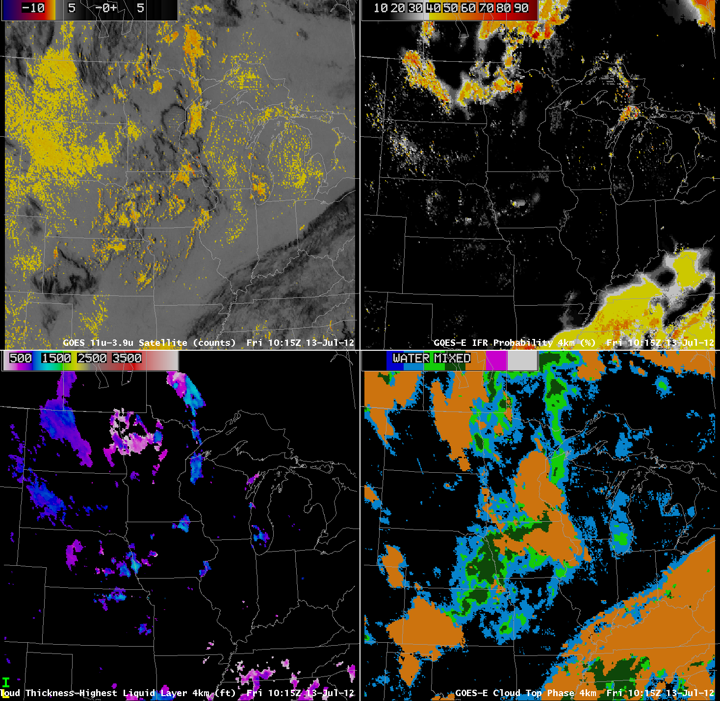
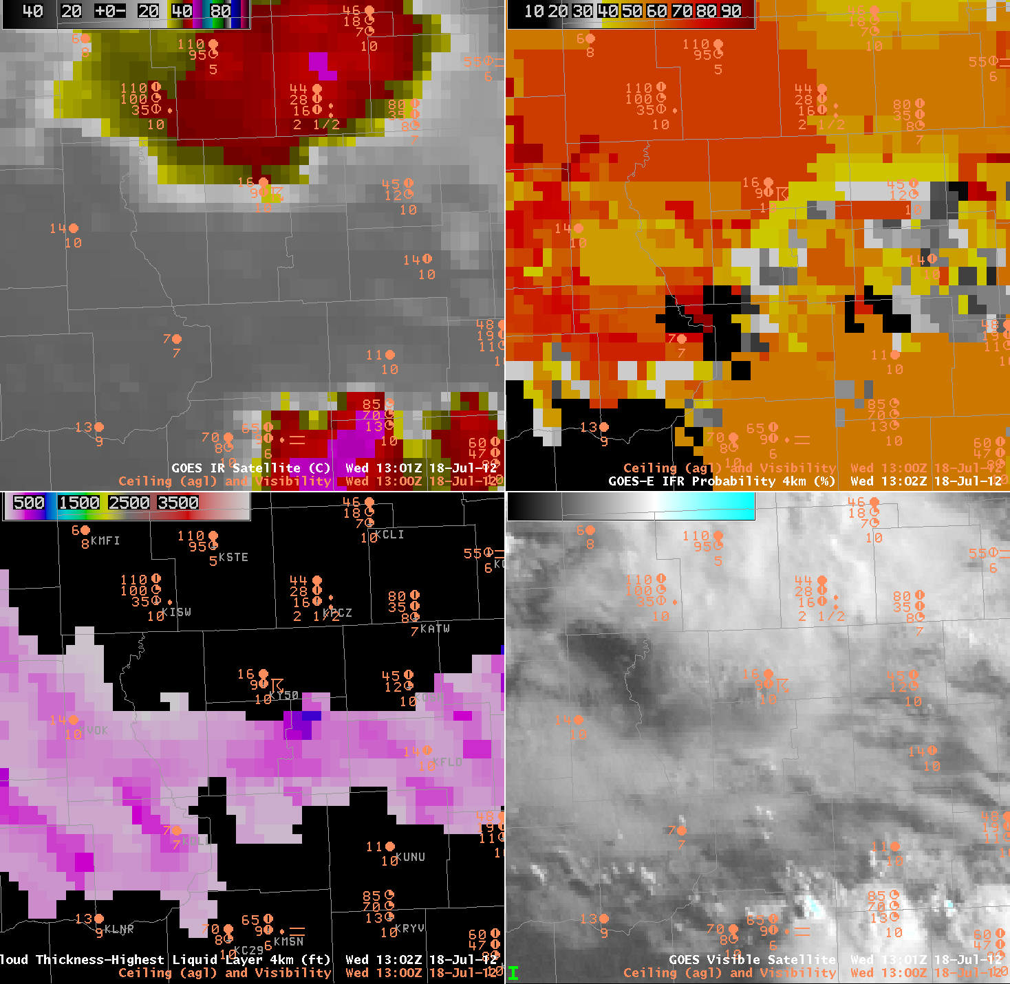
GOES-East Enhanced 10.7-micrometer imagery (Upper left), GOES-R IFR Probability (upper right), GOES-R Cloud Phase (lower left), GOES-East Visible imagery (lower right)

This blown-up version of satellite-based (and fused) products over central Wisconsin on the morning of 18 July 2012 shows how the use of different predictors in the GOES-R IFR probability field can be discerned from the character of the field produced.  This was a morning with MVFR/IFR conditions over central Wisconisin (600-foot ceilings at Marshfield (KMFI) and 700-foot ceilings at Wisconsin Dells (KDLL), for example).   IFR probabilities were high in the regions where IFR conditions were observed, but note how smooth the field is in the northwest and southeast part of the GOES-E IFR probability image.  In the regions under the anvil cirrus (cold cloud-tops as depicted in the 10.7 micrometer image, upper left), the GOES-R IFR Probability algorithm will rely on model data.  In this case, the relative humidity in the RAP forecast has more influence because the high clouds mean the satellite signal is not from a fog/low stratus layer and therefore does not influence the IFR probabiltiies.  The layer relative humidity in the model is likely higher in the northwestern part of the image (where GOES-R IFR probabilities are in the 70% range) than in the southeastern part of the image (where GOES-R IFR probabilities are in the 50% range).  Over the central part of the GOES-R IFR Probability image, the absence of high clouds allows satellite information to be used, and a more variable field results that has a mirror in the variability of the satellite observations in that area.  This region is also where Cloud Thickness diagnoses can be made.

GOES-R Cloud Depth

GOES-East Brightness Temperature Differences (upper left), GOES-R Fog/Low Stratus IFR Probabilities (upper right), GOES-R Cloud Thickness (lower left) and Cloud-top Phase (lower right) on Friday 13 July 2012 at 10:15 UTC

 The figure above shows cloud thicknesses around 1000 feet near Omaha, Nebraska, in a region where cloud phase products suggest water clouds and supercooled clouds with small patches of cirrus, suggestive of clouds that might not be stratiform.  The cloud thickness algorithm (the algorithm predicts the depth of the highest liquid layer) works night and day, although not in times of twilight.

Note also in the image the many false positives in the traditional brightness temperature difference product over South Dakota.  This region shows very low IFR probabilities, in contrast to the region over North Dakota where IFR probabilities are higher and where fog/low stratus is more likely, given the satellite image from 1125 UTC below.  None of the widely-spaced stations in the Dakotas reported IFR conditions;  there were some reports in northwestern Minnesota, however.

Visible GOES-East image, 1125 UTC on 13 July, with a low-light enhancement applied.

 At 1315 UTC, during daytime, cloud thickness products show somewhat thinner low clouds in a region of very low IFR probability.  The sounding from Omaha, bottom, suggests convective, not stratiform, clouds are present.  The GOES-R Cloud Thickness product is produced assuming a stratiform cloud, and results are more likely to be erroneous for situations with clouds that are more cumuliform.  Cloud thickness is derived in part by dividing the liquid water path by liquid water content:  for fog and low stratus, the liquid waer content value is 0.06″ per the meteorological literature.  If the clouds are actually non-stratiform, the assumed liquid water content may not be accurate.  Remember that the cloud depth product was designed to augment the fog/low stratus probability to assist in determining how thick the fog is, and therefore how long it will take to dissipate during the day.  Use the cloud depth with caution if the clouds in question are not stratiform.

GOES-East Brightness Temperature Differences (upper left), GOES-R Fog/Low Stratus IFR Probabilities (upper right), GOES-R Cloud Thickness (lower left) and Cloud-top Phase (lower right) on Friday 13 July 2012 at 13:15 UTC
Skew-T/Log-P thermodynamic diagram from Omaha, Nebraska (KOAX) at 1200 UTC on 13 July 2012

Cirrus Effects in GOES-R Fog/Low Stratus Prediction

MODIS-based IFR Probabilities (Upper Left), Cloud Thickness of the Highest Liquid Layer (Upper Right), 3.7 micron brightness temperatures (Lower Left) and MODIS Cloud Phase (Lower Right) from 1100 UTC on 12 July 2012.

A benefit of the GOES-R Fog/Low Stratus product is that it provides a signal even in the presence of higher clouds that make fog detection via brightness temperature difference methods impossible.  In this case from 1100 UTC on 12 July, a thin cirrus shield off the coast of Oregon (the bright white wisp in the 3.7 micron imagery in the bottom left) shows up (correctly) as an ice cloud in the cloud phase field (bottom right).  Note that low cloud thickness is not computed when higher clouds overlay the low cloud field — so data are available underneath the cirrus deck, although you might infer the thickness from the surrounding fields.  The GOES-R IFR probabilities show values exceeding 50% underneath the cirrus deck, in a region where the brightness temperature difference gives no information.

This effect is also seen in GOES-based imagery, below, from 1200 UTC.  The Cirrus cloud has moved onshore just south of KONP (Newport, OR) where IFR conditions exist.  The IFR probabilities suggest fog/low clouds are likely present in a region where the brightness temperature difference field gives no information because of cirrus clouds.  Although this cirrus shield is small, it should be easy to envision a larger cirrus shield and what that impact might be.

Note also the number of false positives in the brightness temperature difference field that do not show up in the IFR Probabilities.

GOES-West-based Cloud Thickness of the Highest Liquid Layer (Upper Left), IFR Probabilities (Upper Right), 11 micrometer – 3.9 micrometer brightness temperature difference (Bottom Left) and Cloud Phase (Bottom right)

Pacific NW Fog Event

The image above shows IFR probabilities (upper left), Cloud depth (upper right), Cloud type (lower left) and enhanced brightness temperature differences (11 microns – 3.7 microns) for a Puget Sound Fog Event on 11 July 2012.  Heightened IFR probabilities occur where surface observations show IFR conditions are present.

Cloud depths at KUIL, on the coast of Washington are around 800 feet.   The sounding from 72797, below, shows a saturated region between 962 mb and 949 mb.  This is equivalent to a depth (using the hypsometric equation and a mean Temperature in the layer of 13.4 C) of 114 m.  If the cloud bases extend down to 980 mb — a possibility — then the layer depth would be about 270 m.  Note that the MODIS imagery is not at 1200 UTC, the time of the sounding.

GOES data can also be used to produce Fog/Low stratus products.  The GOES Image from the same time, below, shows similar patterns as the MODIS imagery, with the expected differences due to GOES’s inferior resolution.  In particular, GOES has difficulties detecting small spatial variability in fog that arises due to river valleys.  Note also that the cloud depth at 1015 UTC from GOES shows good agreement with the MODIS product:  values are around 900-1000 feet.  These values persist through 1200 UTC (the nominal time of the sounding) and beyond.

Note in the Cloud Phase product at night the difficulties inherent in detecting low water clouds over the ocean.  Those regions off the coast of Washington are not in fact clear, and both the brightness temperature difference and GOES-R Fog products correctly show fog or low stratus in those areas.

After sunrise, above (the images at 1430/1500 and 1630/1700 UTC), a couple of things change and are noteworthy.  First, the Cloud Top Phase product becomes more complete over the ocean as visible data is incorporated into the algorithm.  Incorporation of visible data reduces Fog/Low Stratus probabilities over the Puget Sound however, even as visible imagery shows persistent clouds there, and adjacent observations (KCLM/Pt. Angeles, for example) show continued IFR conditions.  This may be related to non-uniformity in the horizontal in the visible imagery.