Category Archives: Appalachia

Valley Fog in Pennsylvania

VIIRS_20130821_0658

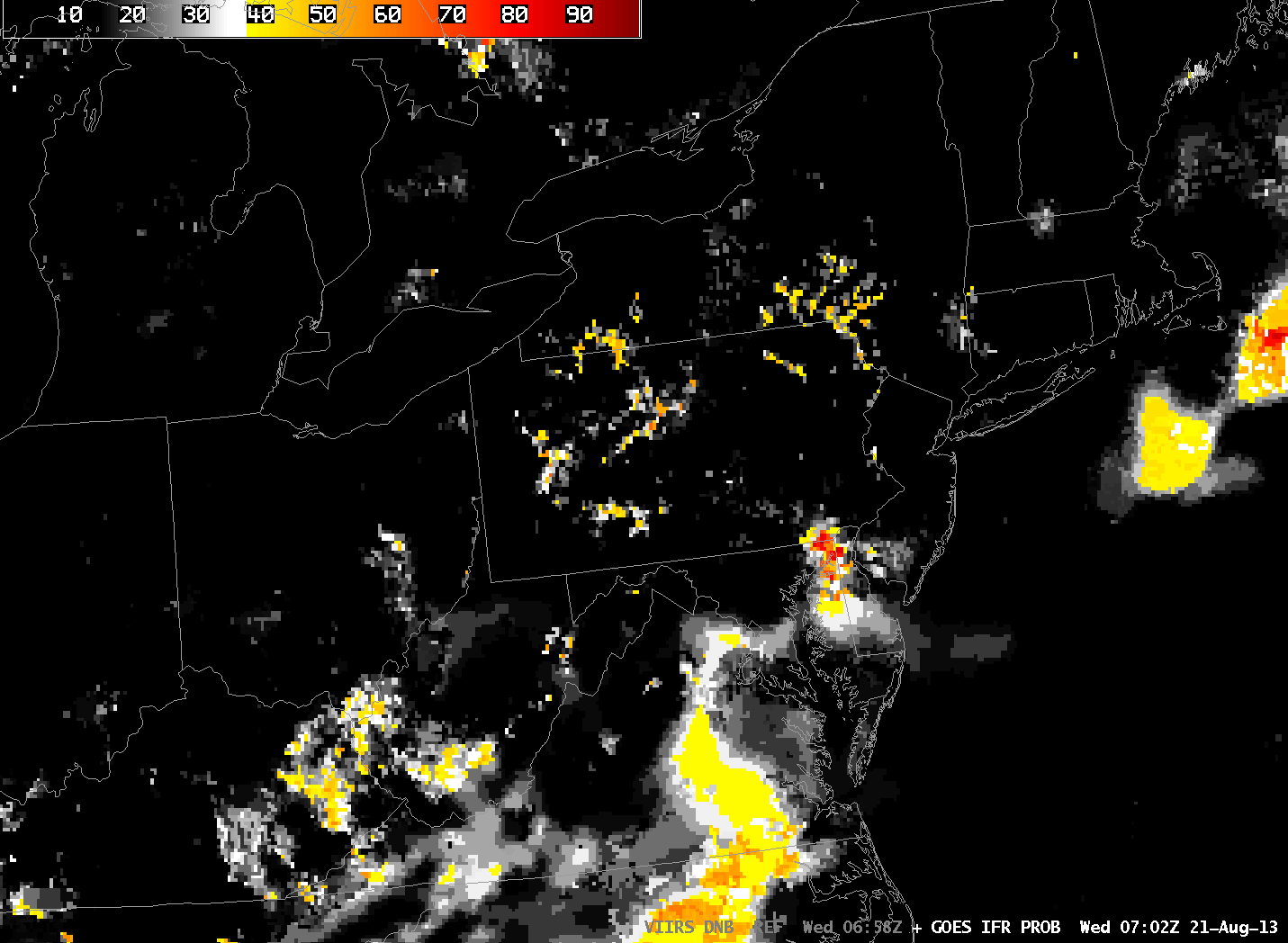
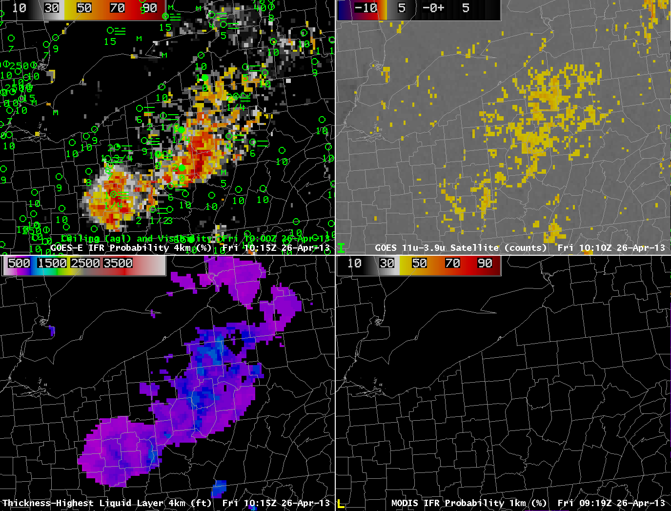
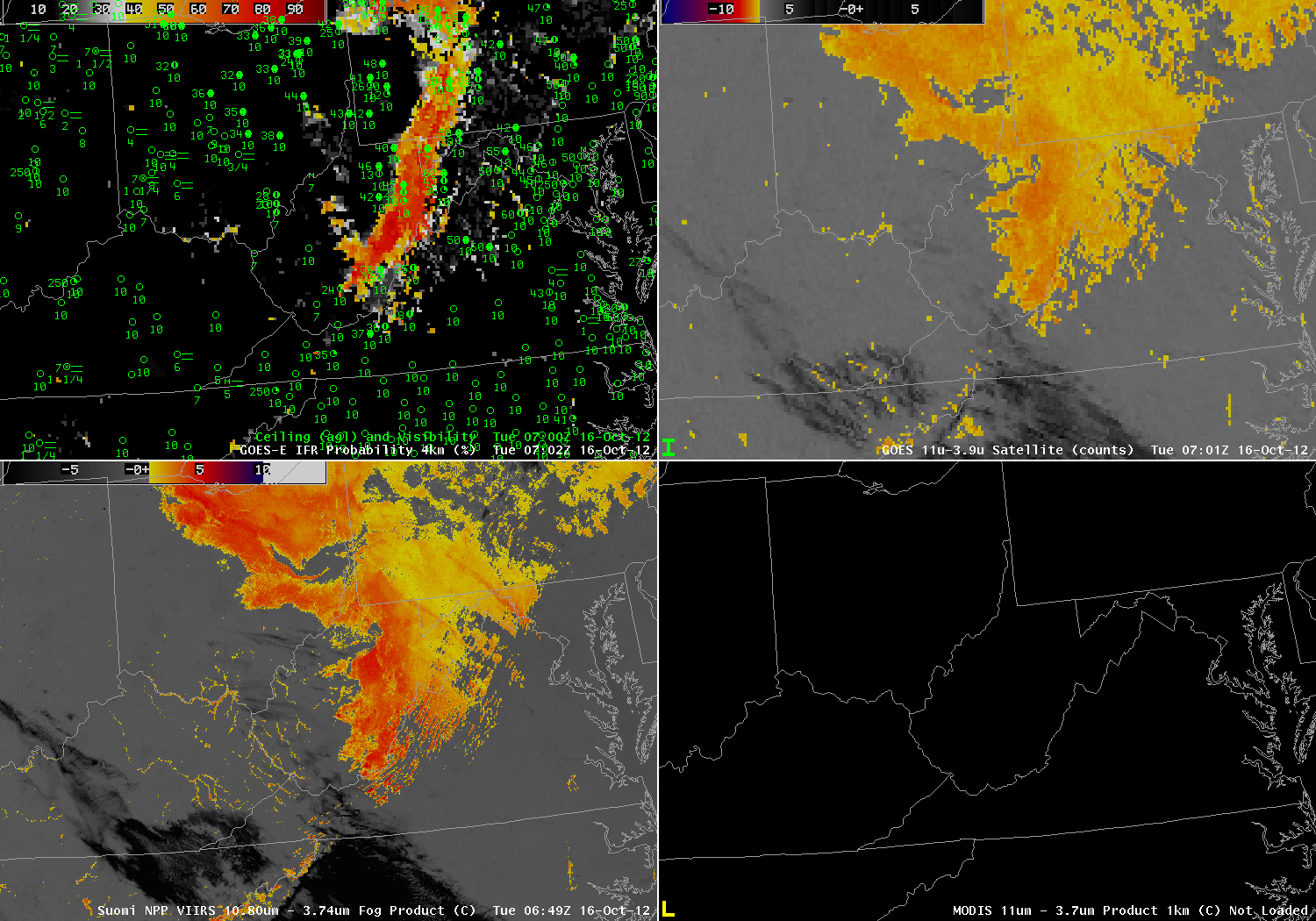
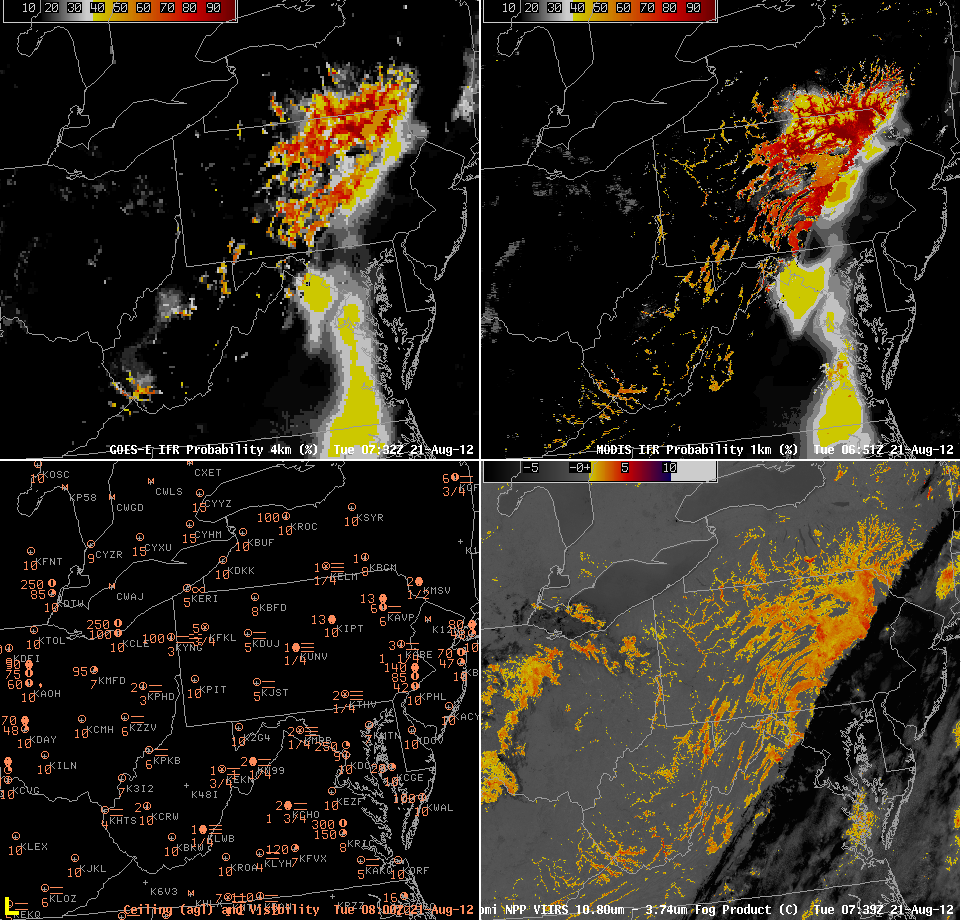
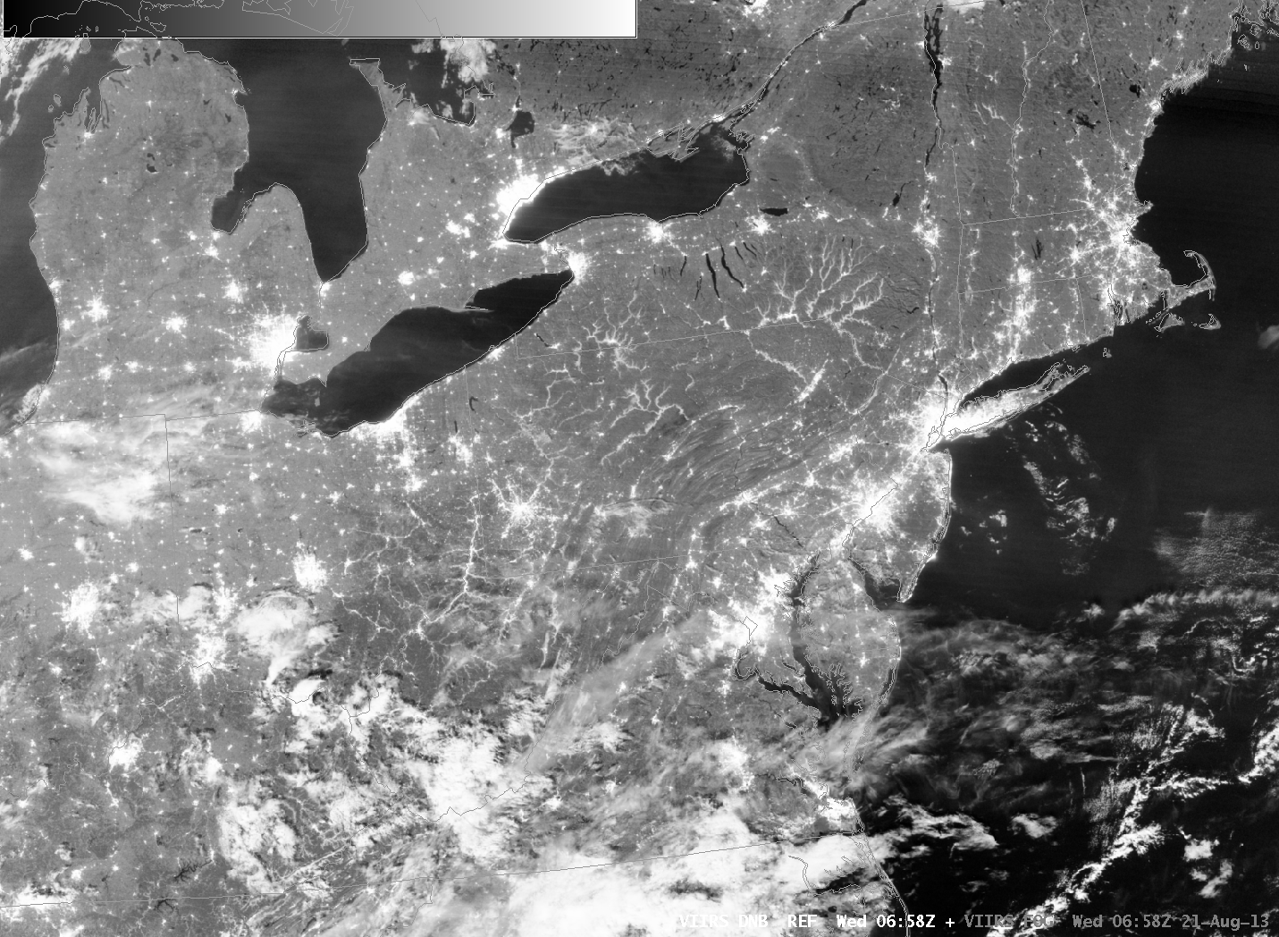
The above animation bewteen the Suomi/NPP VIIRS Day/Night Band and the brightness temperature difference between the longwave infrared image and the shortwave infrared image (that highlights water-based clouds because of emissivity differences at the two wavelengths) shows fog/low stratus in the river valleys of Pennsylvania. The high spatial resolution of Suomi/NPP allows remarkable detail, and the near-Full Moon provides ample illumination. How well did more conventional satellite imagery depict the developing fog? The GOES-13-based IFR Probability Field, below, shows relatively high values in regions over Pennsylvania that are near the river valleys, but GOES lacks the spatial resolution to portray adequately the horizontally confined river valley fog — although someone with knowledge of Pennsylvania Geography can infer a lot.

GOES_IFR_PROB_20130821_0702

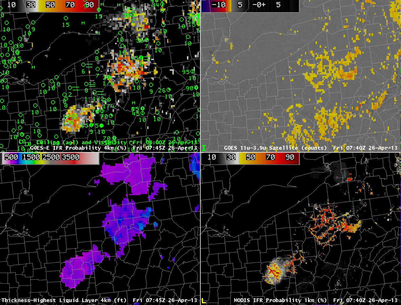
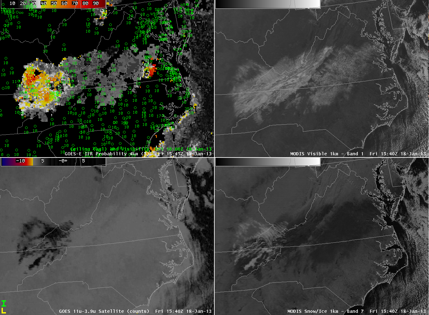
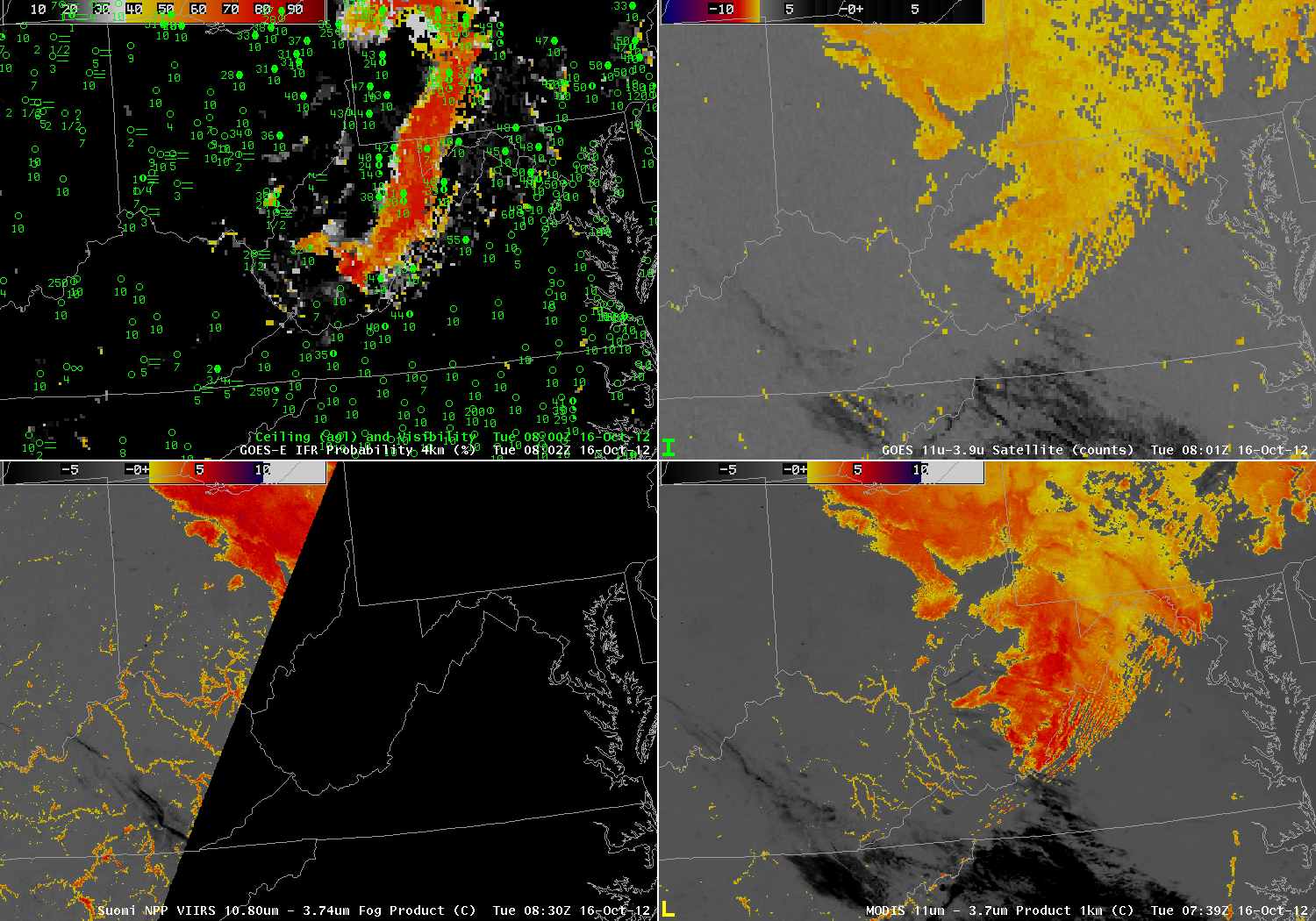
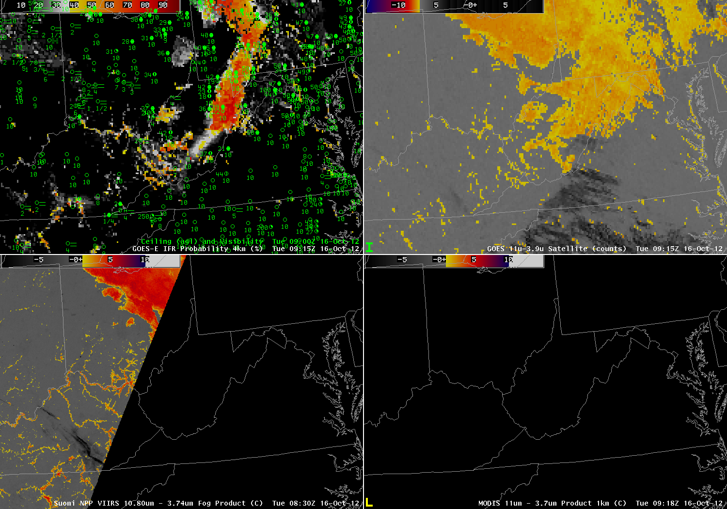
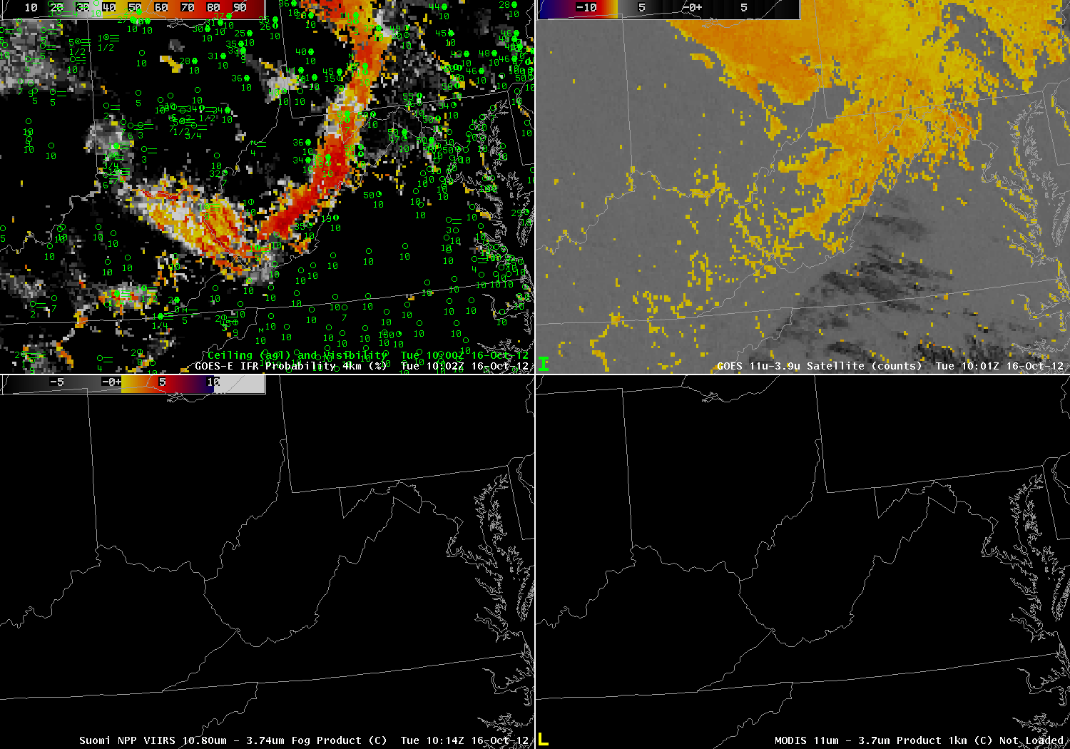
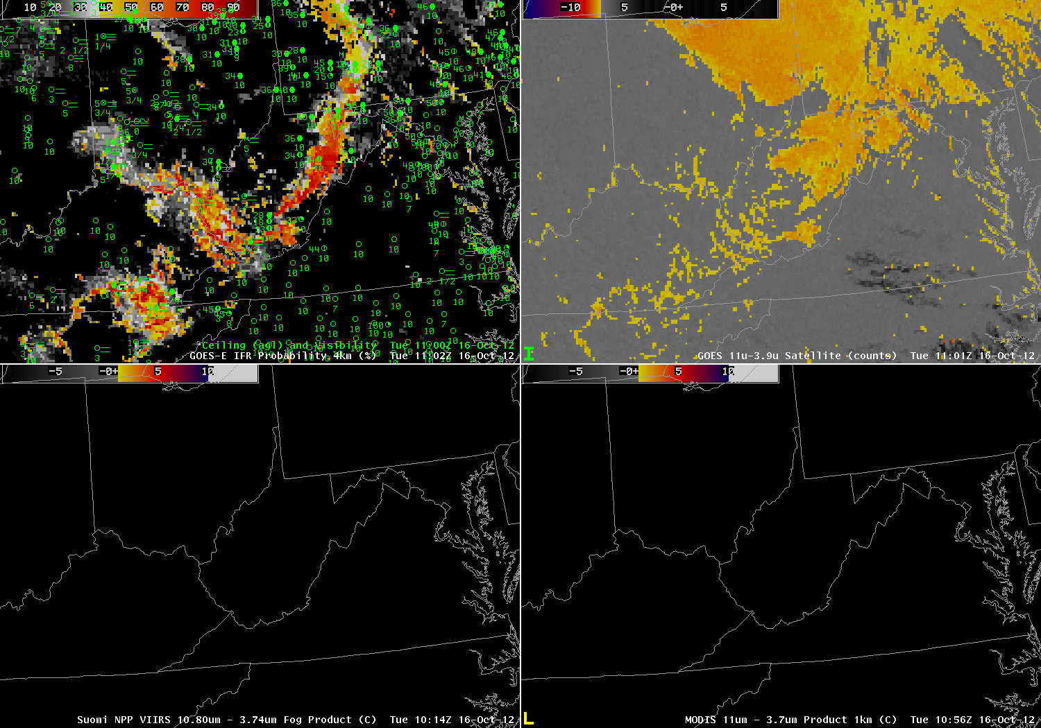
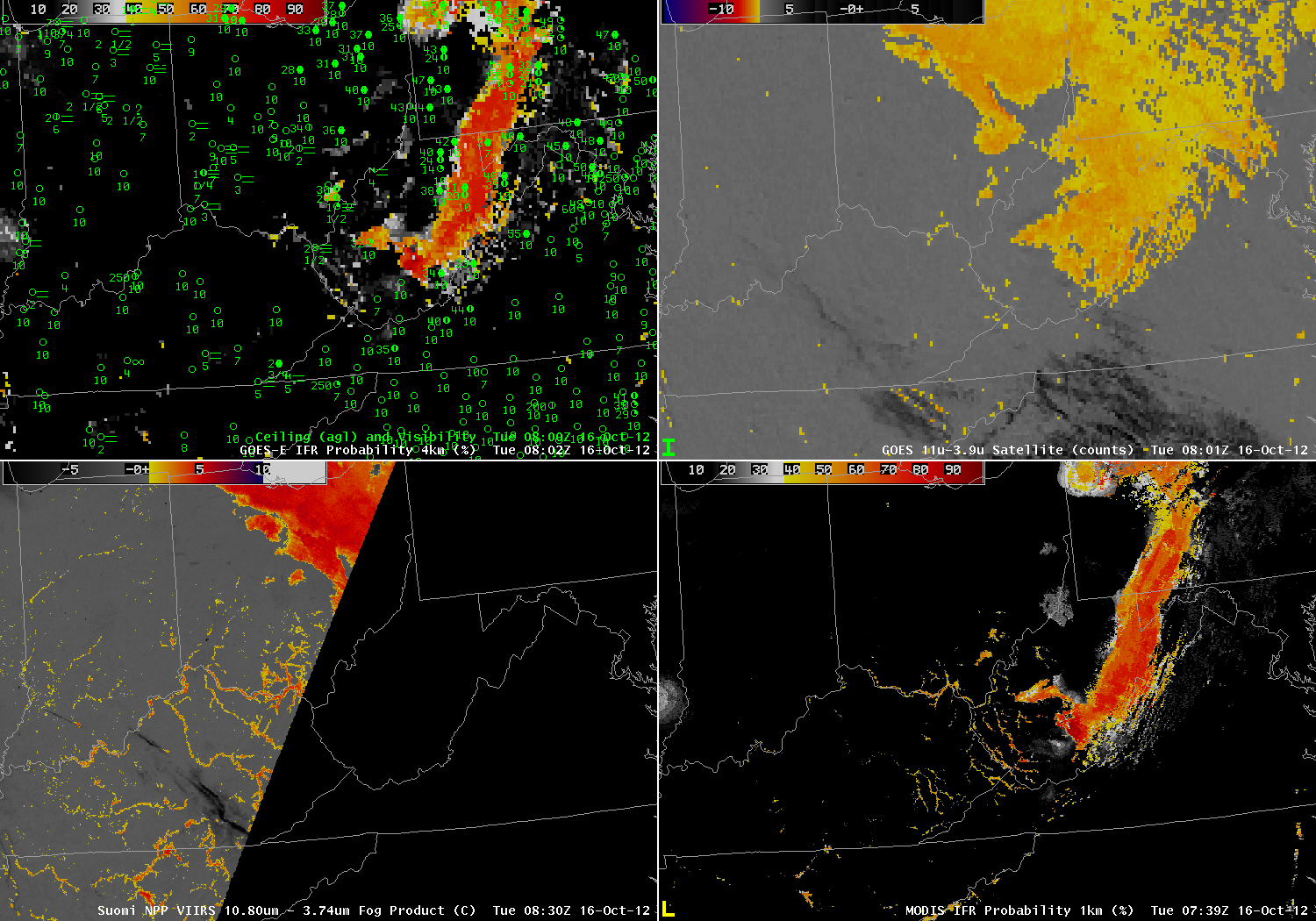
The strength of GOES imagery is temporal consistency and 15-minute timesteps. Polar orbiter data can only give occasional looks. For example, MODIS Imagery can be used to generate brightness temperature differences and IFR Probabilities, below, but they are produced only every 90 minutes at most (although they will still give useful information, even at the edges of the MODIS swath where resolution is degraded).

MODIS_FOG_20130821_loop

MODIS_IFR_PROB_20130821_loop

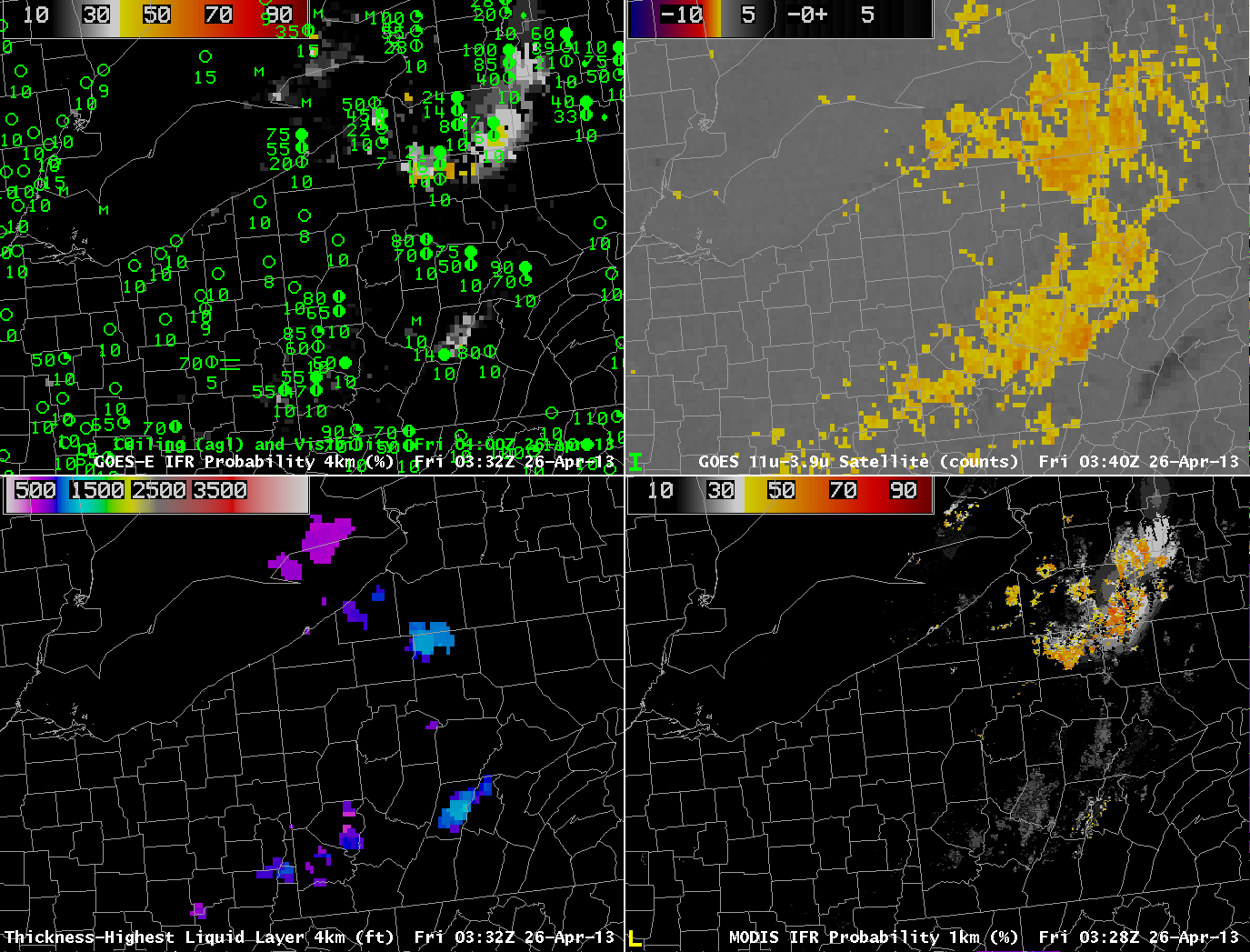
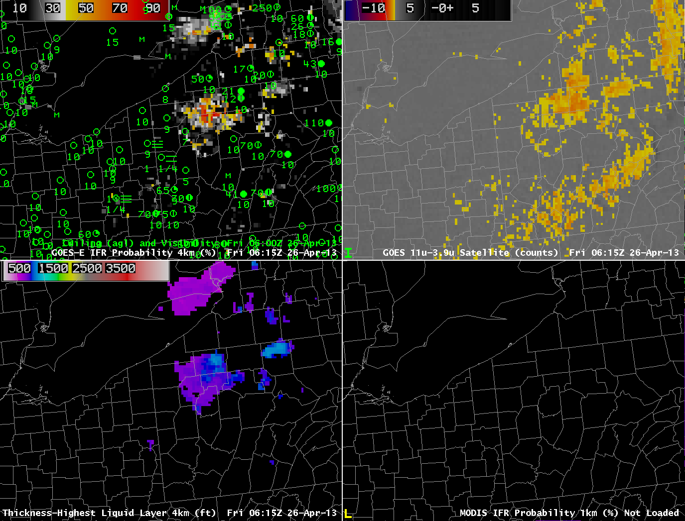
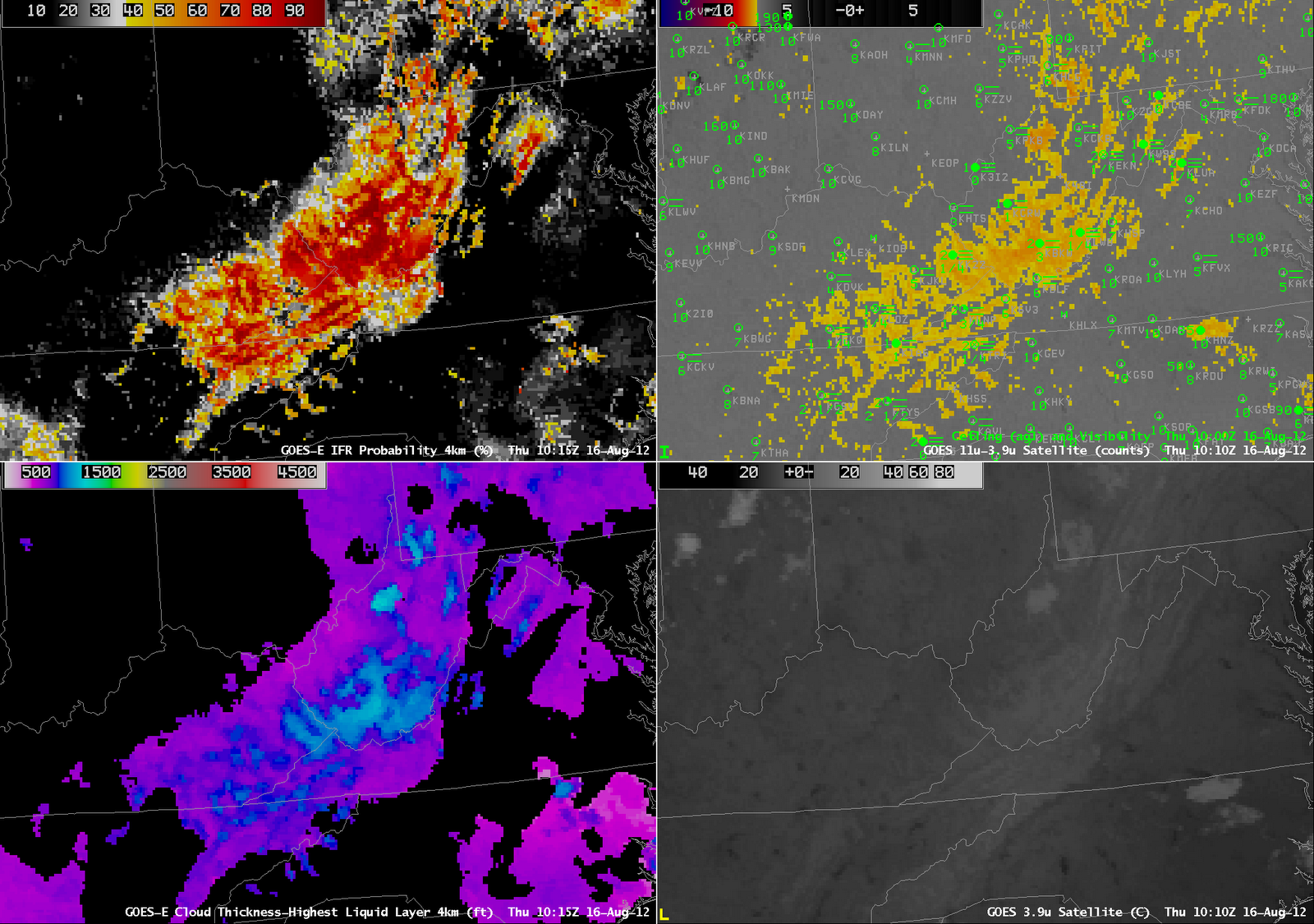
The animation of IFR Probabilities from GOES-East, below, nicely depicts the slow increase in Valley Fog. This animation in concert with knowledge of the geography, augmented with the occasional high-resolution imagery from polar orbiters, as above, should allow a forecaster to describe the location of fog development overnight.

GOES_IFR_PROB_20130821_loop

Visible imagery, below, shows the dissipation of the fog during the morning of August 21st.

GOES13_VIS_21AUG2013loop

Fog was also abundant over Pennsylvania the morning of 20 August. GOES-14, in SRSO-R mode, captured the dissipation. Link. (Courtesy Dan Lindsey, NOAA).

What does MODIS-type Resolution get you?

MODIS-based IFR Probabilities and Cloud Thickness, 0657 UTC on 15 August 2013

MODIS-based IFR Probabilities and Cloud Thickness, 0657 UTC on 15 August 2013

The 1-km data available from the MODIS (above) that is on the Terra and Aqua satellites allows much better resolution than the nominal 4-km resolution from GOES-East and GOES-West (below). The higher resolution on MODIS yields better depiction of dendritic valley fog patterns in mountainous regions. Extremes in cloud thickness will be deeper with MODIS data as well. (In this example, MODIS-based cloud depths reach 1300 feet, vs. 900 feet in GOES) In addition, because fog/low stratus generally starts at small scales and grows in size, MODIS is more likely to detect the early stages of fog (if a serendipitous overpass occurs). Thus, a forecaster can be alert to subsequent development in the GOES data with its better temporal resolution.

GOES-based IFR Probabilities and Cloud Thickness, 0657 UTC on 15 August 2013

GOES-based IFR Probabilities and Cloud Thickness, 0702 UTC on 15 August 2013

Resolution: GOES vs. MODIS and Suomi/NPP over Appalachia

Brightness Temperature Difference (11µm – 3.74µm) at 0621 and 0750 UTC on 20 June 2013.  Data from VIIRS instrument on Suomi/NPP
Brightness Temperature Difference (10.7 µm – 3.9 µm) at 0625 and 0755 UTC on 20 June 2013.  Data from Imager GOES-East.

The GOES Imager, with a nominal (sub-satellite point) resolution of 4 km, has trouble detecting fog when that fog forms over very narrow valleys, as are common over the central Appalachians of the eastern United States.  Compare the views from the GOES Imager (the bottom images) to the view from the Suomi/NPP VIIRS instrument that has 1-km resolution.  VIIRS is much better able to capture the dendritic nature of valley fog, and also to detect it at all when the horizontal scale is very small (for example, the southwest-to-northeast oriented valleys in extreme southwest Virginia).  Thus, a signal will appear first in the high-resolution 1-km polar orbiter data, sometimes several hours before it appears in the coarser-resolution GOES Imager data.

These resolution issues that are apparent in the Brightness Temperature Difference fields, above, the traditional method of detecting fog and low stratus, carry over to the GOES-R IFR Probability fields.  Imagery below, from 0745 UTC on 20 June 2013 suggests that the higher-resolution MODIS data better captures the structure of fog in mountain valleys.  Note also the horizontal shift in the field that occurs because of the GOES parallax shift.

GOES-R IFR Probability fields computed from GOES-East and from Aqua MODIS data, 0745 UTC on 20 June 2013

Radiation Fog over the Allegheny Mountains of Pennsylvania

GOES-R IFR Probabilities computed using GOES-East data, hourly from 0400 UTC through 1000 UTC (excluding 0500 UTC), 26 April 2013

GOES-R IFR Probabilities show a region over the Allegheny Mountains of northwest Pennsylvania slowly acquiring higher and higher probabilities, as ceilings and visibilities drop.  How did this product perform relative to traditional fog detection imagery (the brightness temperature difference product) and relative to data from Polar Orbiting satellites?  (The 0500 UTC imagery is excluded from the animation above because Stray Light Contamination in the 3.9 channel was apparent in the IFR probability fields).

GOES-R IFR Probability computed from GOES-East, 0332 UTC (Upper Left), GOES-East Brightness temperature Difference field (10.7µm – 3.9µm) at 0340 UTC (Upper Right), GOES-R Cloud Thickness (Lower left), GOES-R IFR Probability computed from MODIS data, 0328 UTC (Lower Left).

The ‘traditional’ method of fog detection that exploits emissivity difference of water clouds at 10.7µm and 3.9 µm, upper right in the figure above, at about 0330 UTC, just as the radiation fog was starting to develop, shows clouds detected over north-central Pennsylvania, but also from Centre County southwestward to the Laurel Highlands and to West Virginia.  GOES-based and MODIS-based IFR Probability fields have very low probabilities with these primarily mid-level clouds.

As above, but at 0615 UTC 26 April 2013

By 0615 UTC, IFR probabilities continue to increase over north-central Pennsylvania, and they remain low over southern and central Pennsylvania where mid-level clouds are reported (4100-foot ceilings at Johnstown, for example).

As above, but at 0740 UTC 26 April 2013

Another MODIS overpass at 0740 UTC better resolves the character of the developing fog and low stratus over north-central Pennsylvania.  Very high IFR probabilities in the MODIS-based fields outline the river valleys of the Allegheny Plateau in north-Central Pennsylvania.  GOES-based IFR Probabilities are high, but GOES lacks the resolution to view clearly the individual river valleys.

As above, but with Suomi/NPP brightness temperature difference (10.8 µm- 3.74µm) and Day-Night Visible imagery in the bottom right (0652 UTC), with the GOES-R IFR Probabilities (Upper Left), GOES-E Brightness Temperature Difference field (Upper Right), and GOES-R Cloud Thickness toggling between 0645 and 0702 UTC.

Suomi/NPP can also give information at high resolution about the evolving fog field.  The tendrils of fog developing in the river valleys are evident in the visible imagery created using reflected lunar illumination (A mostly full moon was present the morning of 26 April) and those water-based clouds are also highlighted in the Suomi/NPP Brightness Temperature Difference Field.  The clouds over the Laurel Highlands are higher clouds — they are casting shadows visible in the Day/Night band.

As in the figure above, but for 1015 UTC 26 April 2013

The final GOES-R Cloud Thickness field before twilight conditions, above, shows maximum thicknesses of 900 feet over Warren County, Pennsylvania, and around 850 feet over southern Clarion County.  According to this link, such a radiation fog will burn off in less than 3 hours after sunrise.  The animation below of visible imagery at 1315 and 1402 UTC shows the fog, initially widespread in river valleys at 1315 UTC mostly gone by 1402 UTC.

GOES-13 Visible Imagery, 1315 and 1402 UTC, 26 April 2013.  Warren and Clarion Counties are highlighted.

Fog-related Crash on I-77 in southern Virginia

GOES-R IFR Probabilities computed from GOES-East (Upper Left), MODIS Visible imagery and surface plots of ceilings/visibility (Upper Right), GOES-R IFR Probabilities computed from MODIS (Lower Left), MODIS 10.7 micron data (Lower Right), images at ~1630 and ~1815 UTC.

Seventeen separate crashes involving nearly 100 vehicles near milepost 5 on Interstate 77 in Carroll County in southern Virginia claimed three lives on Sunday March 31st.  The crashes occurred in fog and started around 1 PM (1700 UTC).  How did the Fog/Low Stratus product do in alerting forecasters to the presence of the fog?   This case demonstrates the challenges inherent in Fog Detection.  GOES-R IFR Probabilities show a distinct reduction in probabilities over the crash site in the times bracketing the crash time, above.  An animation of GOES-based IFR probabilities, below, shows relatively high probabilities until just before the crash time, after which time probabilities dropped.  Photographs from after the crash, during the clean-up, show that fog persisted into the afternoon hours.

GOES-R IFR Probabilities computed from GOES-East and Rapid Refresh Data, 1602-1815 UTC on 31 March 2013

Note that widespread fog is typically not associated with crashes.  Rather, patchy fog that can be driven into from regions with greater visibility is a greater hazard.  Such patchy fog is most likely to be sub-pixel scale.

IFR Probabilities over snow

GOES-R IFR Probabilities from GOES-East and surface observations (Upper Left), MODIS visible imagery (Upper Left), MODIS Brightness Temperature Difference (10.7 µm- 3.9 µm) (Lower Left), MODIS Band 7 (2.2 µm )

GOES-R Cloud Type product from 1545 UTC 18 January 2013

GOES-R IFR Probabilities showed values around 20-25% over the fresh snow cover in south-central Virginia in the Piedmont.  Why?  The GOES-R cloud mask sometimes detects clouds where fresh snowfall is present, as shown in the GOES-R Cloud Type product above, especially if the snow mask is not up to date. The GOES-R cloud type product determines the phase of any pixel detected as cloud by the cloud mask;  clouds were detected, albeit incorrectly, in this area and classified as water clouds. It is unlikely that clouds are present over south-central Virginia because the brightness temperature difference product suggests no water-based clouds in this region — the white areas in the visible over southern Virginia and northern North Carolina have a signature in the 2.2 µm channel (lower right in the 4-panel image) that is strongly indicative of snow on the ground (snow strongly absorbs radiation at that wavelength, so little energy is reflected back to the satellite). The GOES-R FLS product is dependent upon the GOES-R cloud mask during the day and calculates the probability that IFR conditions are present for any detected cloudy pixel.  The presence of clouds in the Cloud Type product for reasons stated above leads to the calculation of an IFR probability where clear sky is likely present.  Although the IFR probabilities are higher over the fresh snow than in other clear sky areas, the probabilities are relatively low, around 20-25%. Probabilities in this range should give forecasters low confidence that IFR conditions are present in this area. Conversely, the small region of relatively high IFR probabilities (>50%) in southwest Virginia — near Wakefield — and extreme southwest Virginia — near Wise — correlates well with a region of eroding IFR conditions. Note that cloud ceilings over the mountains of far western Virginia are very close to or below IFR criteria, giving forecasters higher confidence that IFR conditions are present.

GOES-13 Visible Imagery over the mid-Atlantic showing snow cover over Virginia

The Visible imagery above shows generally clear skies over central Virginia, with some cloud streets developing later in the afternoon. The eroding IFR cloud deck over extreme SW Virginia is difficult to see in visible imagery alone but is evident by the dissipating clouds in western Kentucky.

GOES-R Probabilities evolve as the night progresses

GOES-R IFR Probabilities computed from GOES-14 (upper left), GOES-14 heritage brightness temperature difference product (upper right), VIIRS heritage brightness temperature difference product (lower left), MODIS heritage brightness temperature difference product (lower right), all from near 0700 UTC.

MODIS and VIIRS yield satellite information that can be used to detect fog/low stratus at high spatial resolution.  In the exa,ple above, the VIIRS brightness temperature difference product highlights many river valleys as possibly cloud-filled over eastern Kentucky, southern Ohio and southwestern West Virginia.  The coarser resolution of the GOES satellite pixel precludes such fine-scale detection.  Note, however, that both satellite platforms detect the presence of stratiform water clouds over north-central Ohio where surface observations show only mid-level cloudiness.  IFR probabilities are confined to the spine of the Appalachians from the Laurel Mountains near Johnstown (PA) southward towards southern West Virginia.  How do things evolve with time?

As above, but from near 0800 UTC

As above, but from near 0915 UTC

As above, but from near 1000 UTC

As above, but from near 1100 UTC

The power of GOES imagery in this case is to show the evolution of the fog/low stratus field.  Even at this only-hourly timestep, the development of regions of IFR conditions is evident, and those developing conditions occur in tandem with increasing probabilities in the GOES-R IFR Probability field.  Throughout the night, the GOES brightness temperature difference field flags the unimportant (from an aviation standpoint) stratus deck over northcentral Ohio, and the IFR probability field, which field also uses Rapid Refresh Model data, discounts the satellite signal.  By 1100 UTC, the river valley signal has strengthened enough in the GOES imagery to appear, and a corresponding increase in IFR probability occurs.

IFR Probability can also be computed using MODIS data (below). The 0739 UTC MODIS data, shown at the top of this blog post, highlights — as does GOES — the stratus deck over northern Ohio.  The MODIS-based IFR probabilities, however, do not highlight that cloud-deck, by design.  Note also that the higher-resolution MODIS imagery, because it detects river valley fogs at 0739 UTC, also has a strong IFR probability signal there.  Pixel resolution on GOES-R will be intermediate between MODIS and present GOES.

As at top, for near 0800 UTC, but with MODIS-based IFR probabilities in the lower right

Excellent example of the importance of model data

GOES-R IFR Probabilities computed using GOES-East data (Upper Left), GOES-R IFR Probabilities computed using MODIS data (Upper Right), Surface Observations and Cloud Ceilings Above Ground level (Lower Left), Suomi-NPP VIIRS Brightness Temperature Difference field, 10.8  µm – 3.74 µm (Lower Right).  Times as indicated.

Three different satellite sensors — the GOES Imager on GOES-East, MODIS on Aqua, and VIIRS on Suomi/NPP — viewed data from the occurrence of Valley Fog over the Appalachians (and surroundings) early in the morning of 21 August.  A shortcoming of the Brightness Temperature Difference field in the lower left is immediately apparent:  no fog/low stratus is indicated where high clouds exist, even though observations do show IFR conditions.  In contrast, the fused product does show heightened probabilities underneath that high cloud deck.  Probabilities are not as high as they are where both satellite and model predictors can be used to evaluate the presence of fog and low stratus, and the resolution of the field is different, obviously limited to the horizontal resolution of the Rapid Refresh, meaning that small river valleys, that are very obvious in the regions where satellite data are used (and even much more obvious when high-resolution MODIS or VIIRS data are used).  Note also how GOES-R IFR Probabilities de-emphasize the signal over western Ohio, where IFR conditions are not reported.  Brightness temperature difference fields from MODIS and from GOES both see a signal there, as also shown in the VIIRS field, but these stratus clouds are not obstructing visibility.

Bottom line:  MODIS data’s higher resolution observes the big differences between river valleys and adjacent cloud-free ridge tops.  GOES-East has difficulty in resolving those differences.  So MODIS IFR fields better highlight river fog.  Model data can help discern between fog on the ground, and stratus that is off the ground.

Valley Fog over Appalachia

GOES-R IFR Probabilities (Upper Left), Brightness Temperature Difference (10.7 micrometers – 3.9 micrometers) (Upper Right), GOES-R Cloud Thickness (Lower Left), GOES-East 3.9 micrometer imagery (Lower Right)

The radiation fog example over West Virginia and surrounding states on 16 August highlights characteristic strengths of the GOES-R Fog/Low Stratus products.  Note, for example, how the enhanced brightness temperature field shows no apparent signal over the Ohio River Valley along the western border of West Virginia, despite the presence of IFR conditions at Pt. Pleasant (K3I2) and Huntington (KHTS).  In contrast, the IFR probability does the suggest the possibility of visibility obstructions in the valley.

Note the region of low cloud over north-central North Carolina.  The feature is quite apparent in the 3.9-micrometer imagery, and the brightness temperature difference field also has a maximum return there.  This cloud is likely elevated stratus (brightness temperatures were generally in the single digits Celsius), and the IFR Probability field correctly diminishes the strong satellite predictor signal there.