Category Archives: MODIS

The Challenge of Satellite Fog Detection at Very Small Scales

weather-gov-screencapture_1400utc_10nove2016

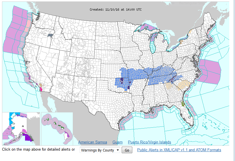
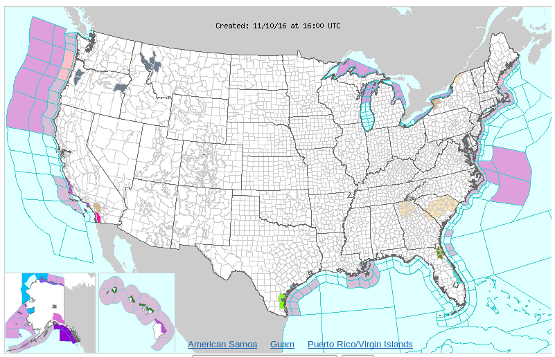
Hazards as depicted by http://weather.gov front page at 1400 UTC on 10 November 2016 (Click to enlarge)

Isolated regions of dense fog developed over eastern Oregon early in the morning on 10 November 2016, and one county — around Baker City — was placed in a Dense Fog advisory (Counties in the Willamette Valley of western Oregon, and near Glacier Park in Montana were placed under Dense Fog Advisories a bit later in the morning on 10 November). Click here to see a 1400 UTC mapping of IFR/LIFR conditions from the Aviation Weather Center.

URGENT – WEATHER MESSAGE
NATIONAL WEATHER SERVICE BOISE ID
600 AM MST THU NOV 10 2016

ORZ062-101800-
/O.NEW.KBOI.FG.Y.0012.161110T1300Z-161110T1800Z/
BAKER COUNTY-
500 AM PST THU NOV 10 2016

…DENSE FOG ADVISORY IN EFFECT UNTIL 10 AM PST THIS MORNING…

THE NATIONAL WEATHER SERVICE IN BOISE HAS ISSUED A DENSE FOG
ADVISORY…WHICH IS IN EFFECT UNTIL 10 AM PST THIS MORNING.

* VISIBILITY…ONE QUARTER MILE OR LESS.

* IMPACTS…TRAVEL HAZARD DUE TO POOR VISIBILITY…ESPECIALLY
ALONG INTERSTATE 84 BETWEEN BAKER CITY AND NORTH POWDER

PRECAUTIONARY/PREPAREDNESS ACTIONS…

A DENSE FOG ADVISORY MEANS VISIBILITIES WILL FREQUENTLY BE
REDUCED TO LESS THAN ONE QUARTER MILE. IF DRIVING…SLOW DOWN…
USE YOUR HEADLIGHTS…AND LEAVE PLENTY OF DISTANCE AHEAD OF YOU.

&&

$$

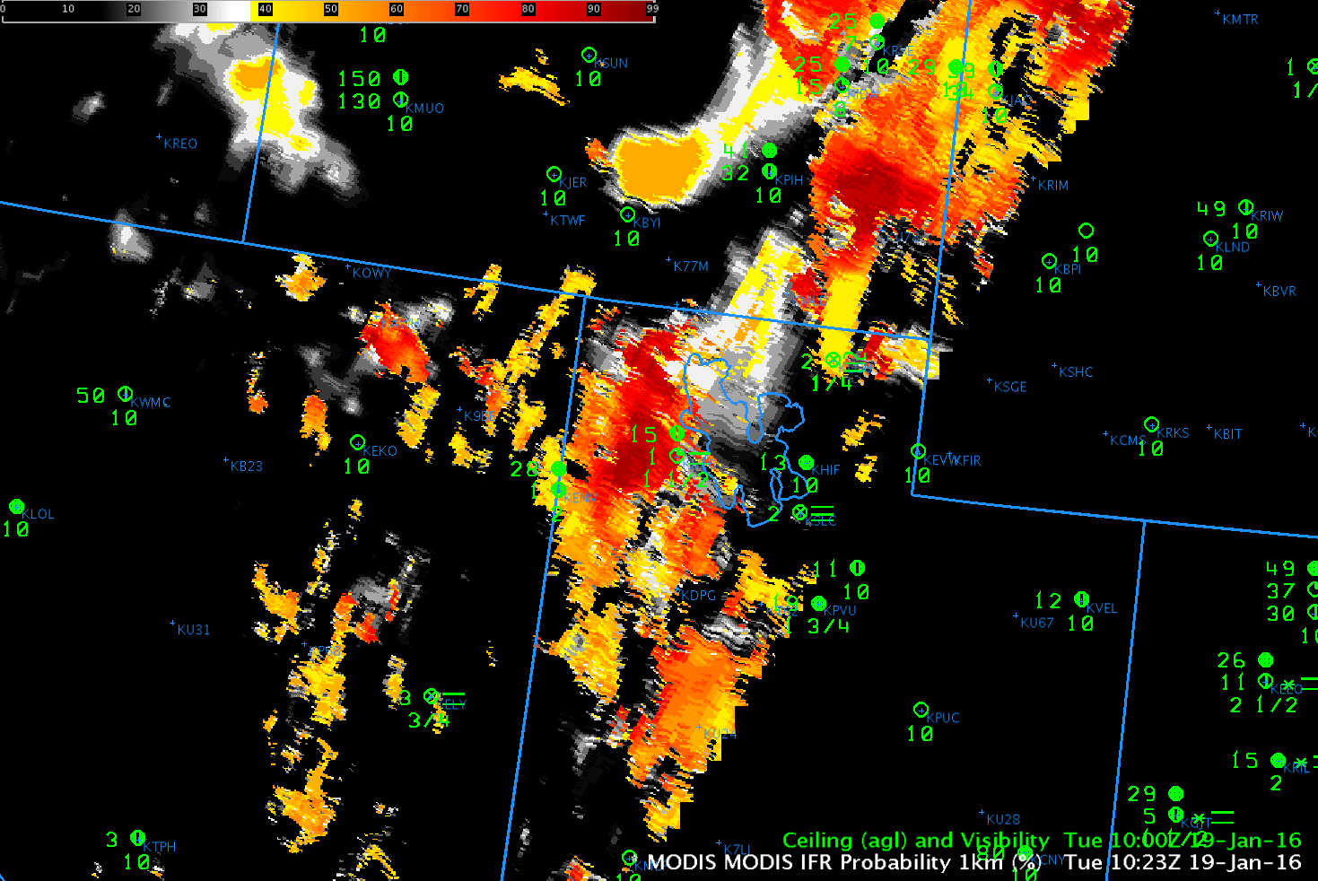
What kind of Fog-detection products are available to assist a forecaster in seeing at a glance that fog is developing? How useful are they for small-scale features such as that in Baker County Oregon?

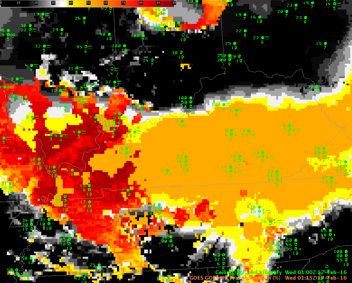
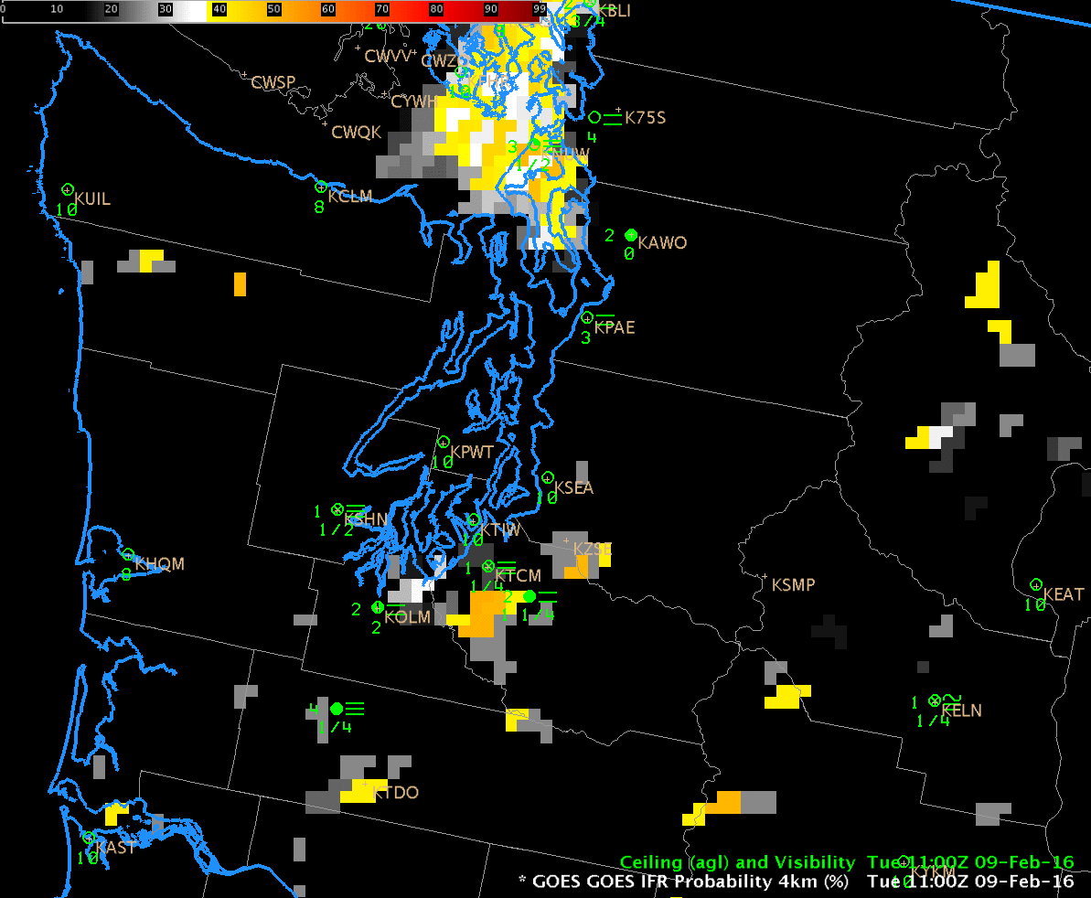
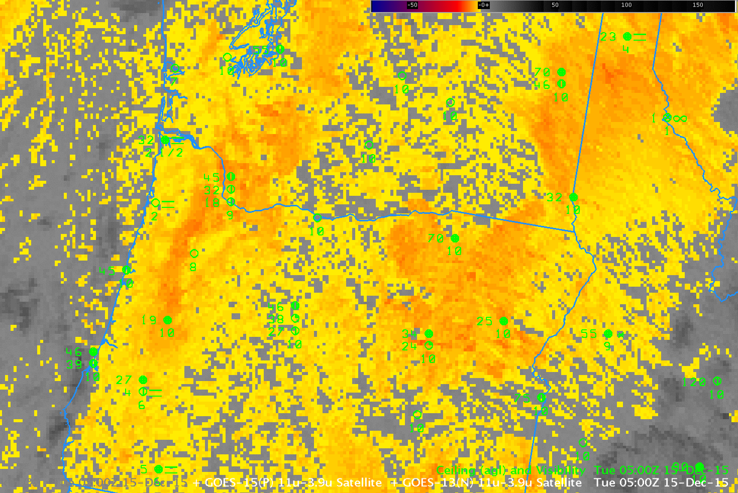
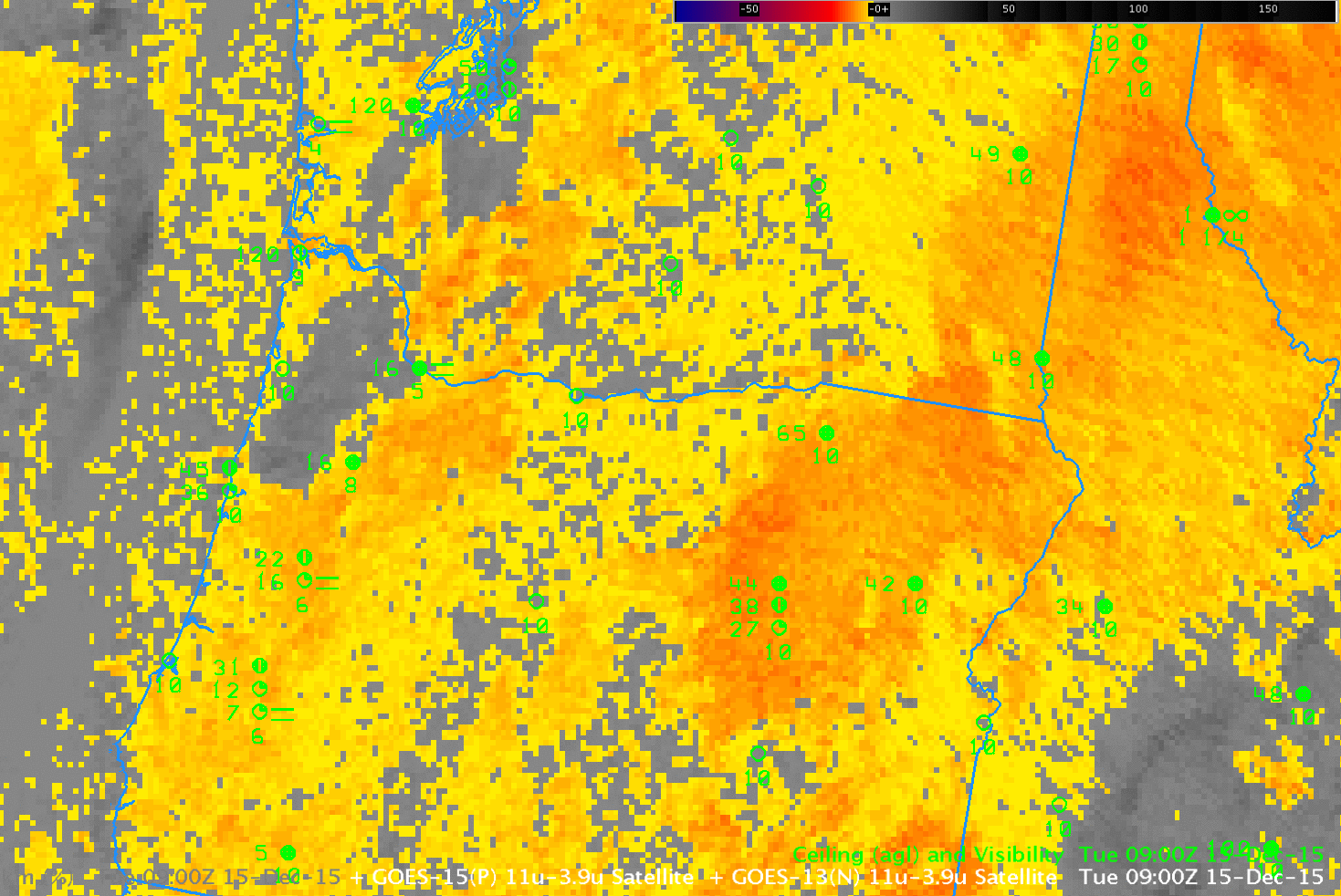
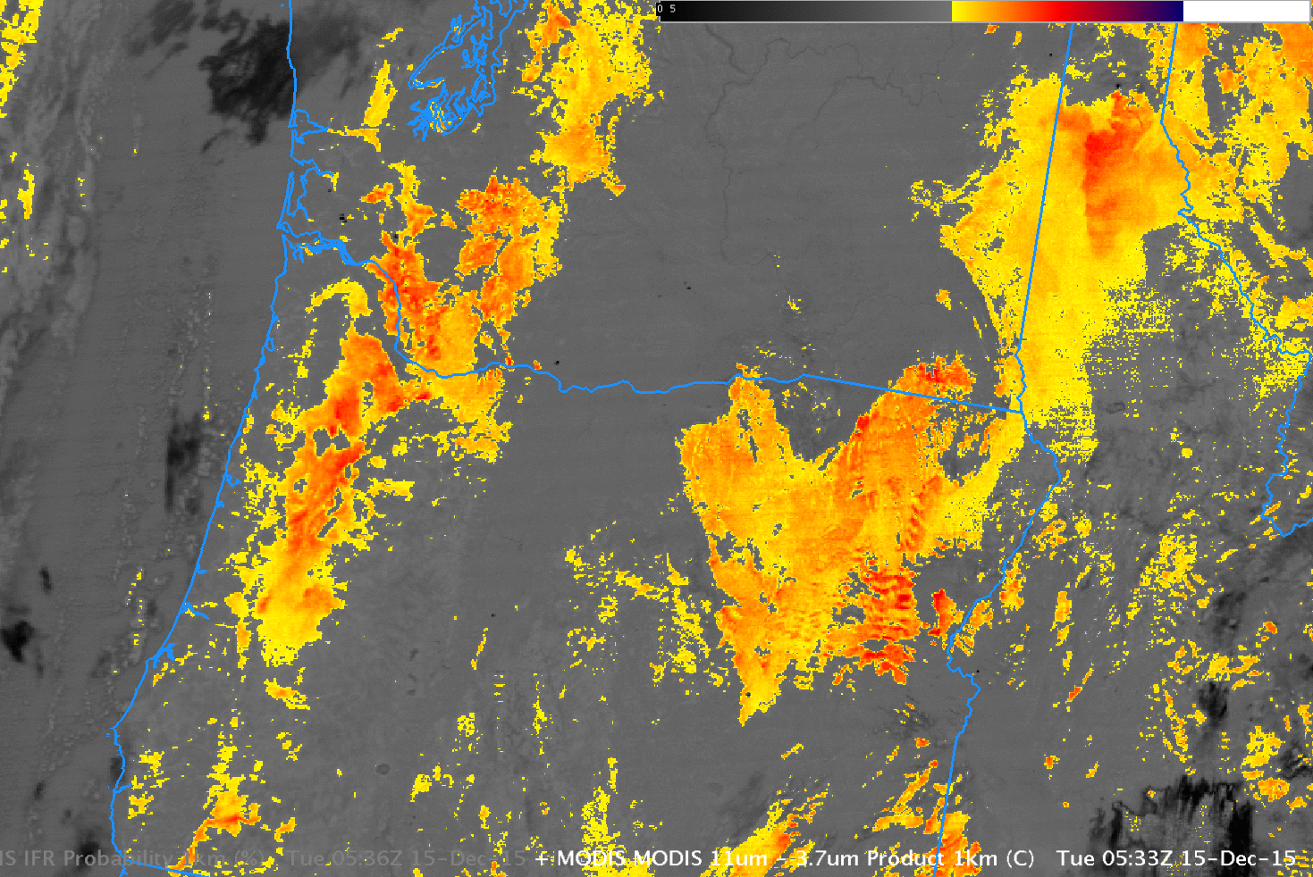
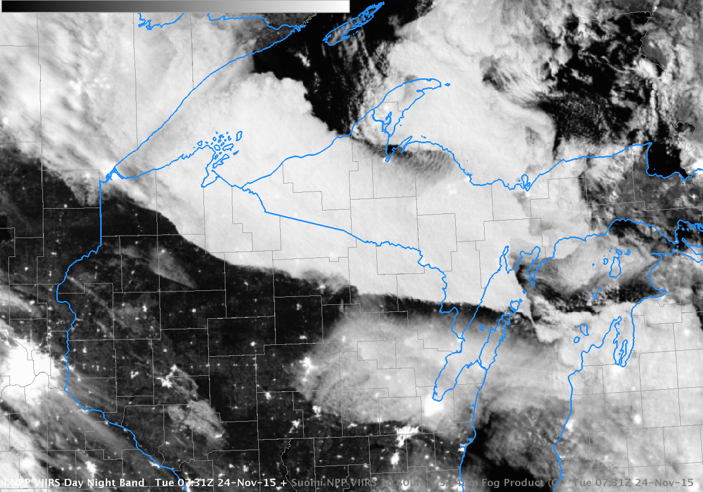
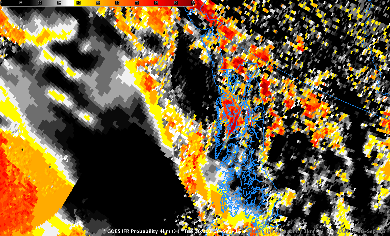
Brightness Temperature Difference Fields (3.9 µm – 10.7 µm) have historically been used to detect fog; the difference field keys on the Emissivity Differences that exist in water-based cloud droplets: they do not emit 3.9 µm radiation as a blackbody, but do emit 10.7 µm radiation more nearly as a blackbody, so computed brightness temperatures are different: cooler at 3.9 µm than at 10.7 µm. The Brightness Temperature Difference fields for 0900 and 1200 UTC are shown below (Note the seam — GOES-13 data are used east of the seam, GOES-15 data are used to the west). There is no distinct signal over Baker County, nor any pattern that can really help identify regions of fog. Cirrus is present over western Oregon (depicted as dark grey or black in this enhancement); satellite-only detection of low fog is not possible if cirrus prevents a view of the surface.

goes15btd_10nov_0900_1200toggle

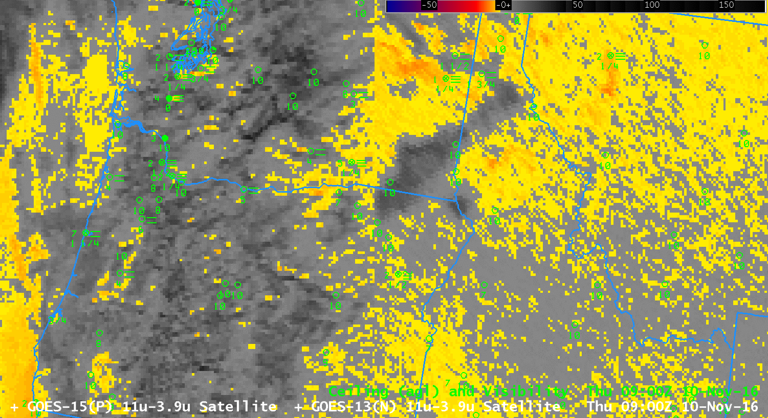
GOES Brightness Temperature Difference Fields (3.9 µm – 10.7 µm) at 0900 and 1200 UTC on 10 November 2016 (Click to enlarge)

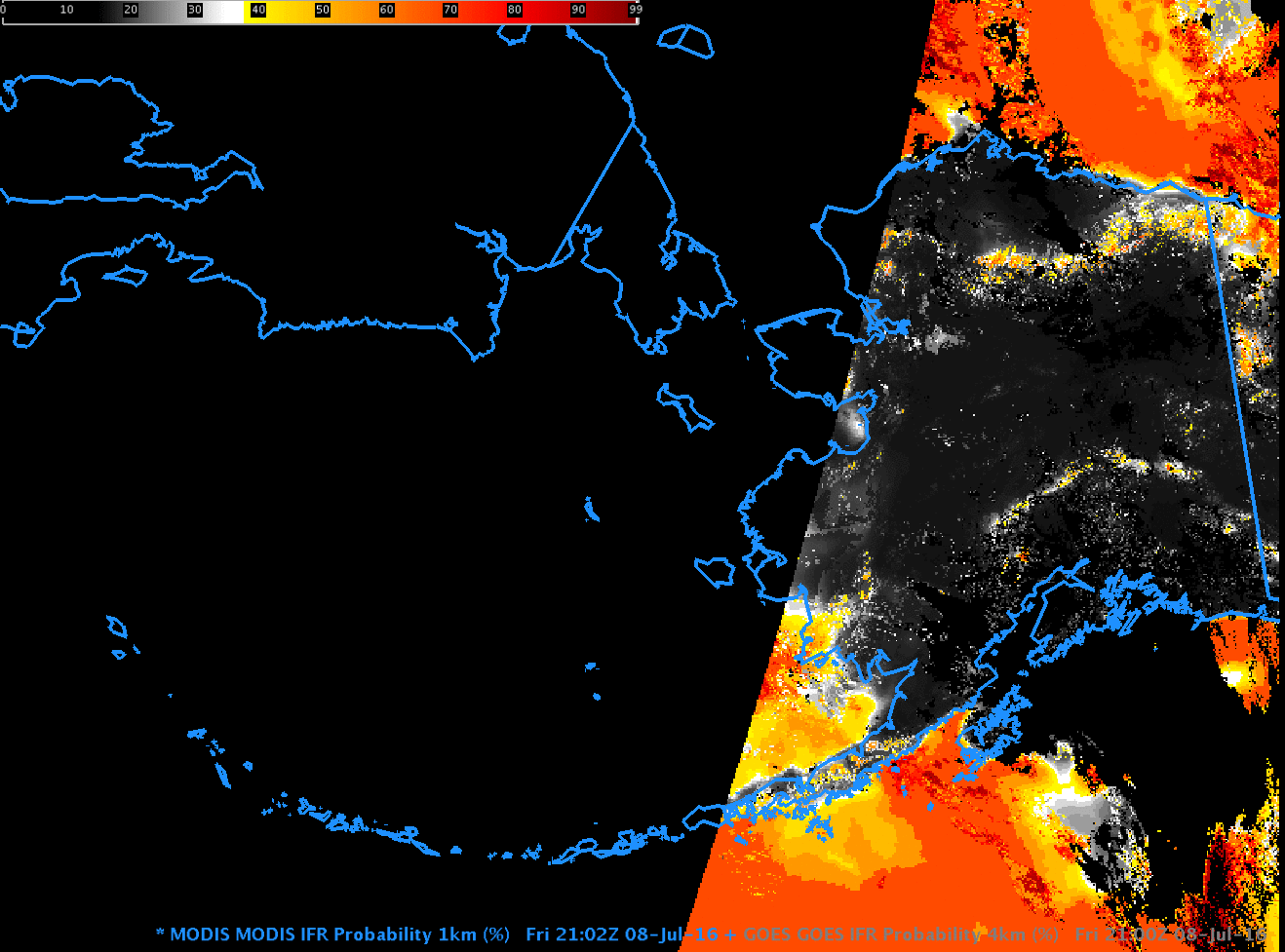
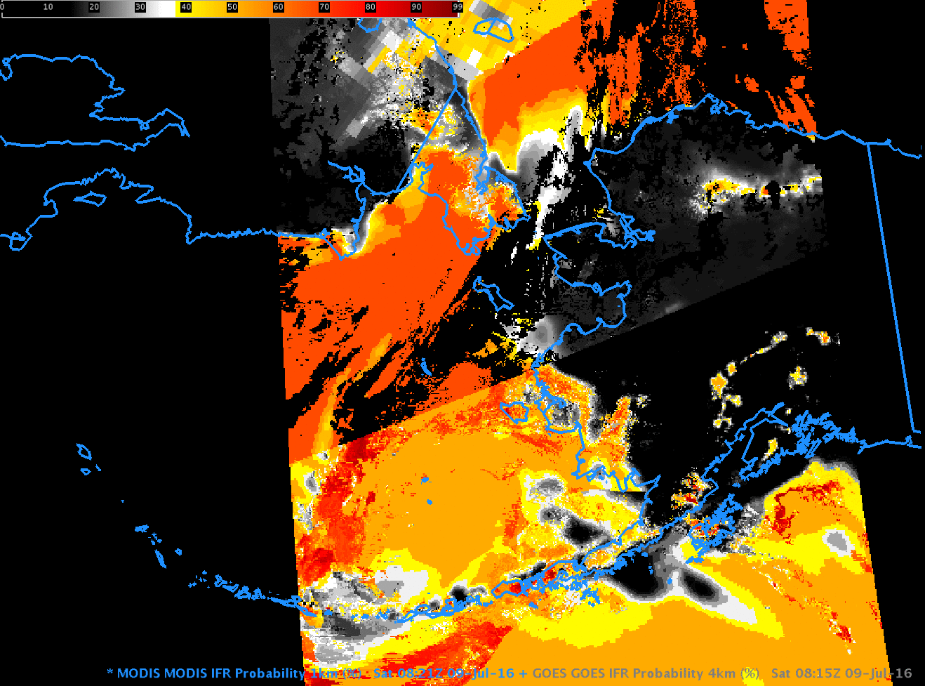
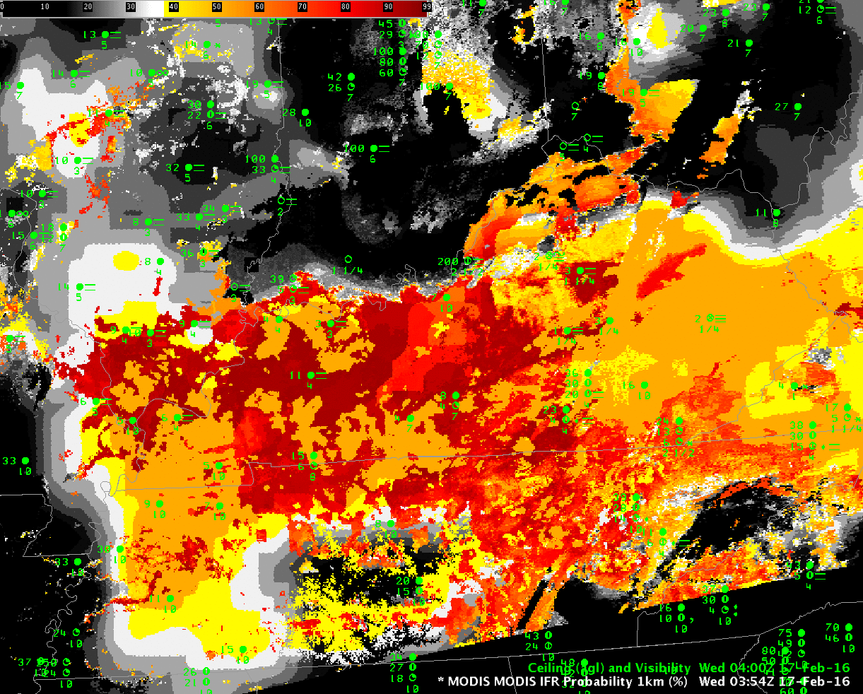
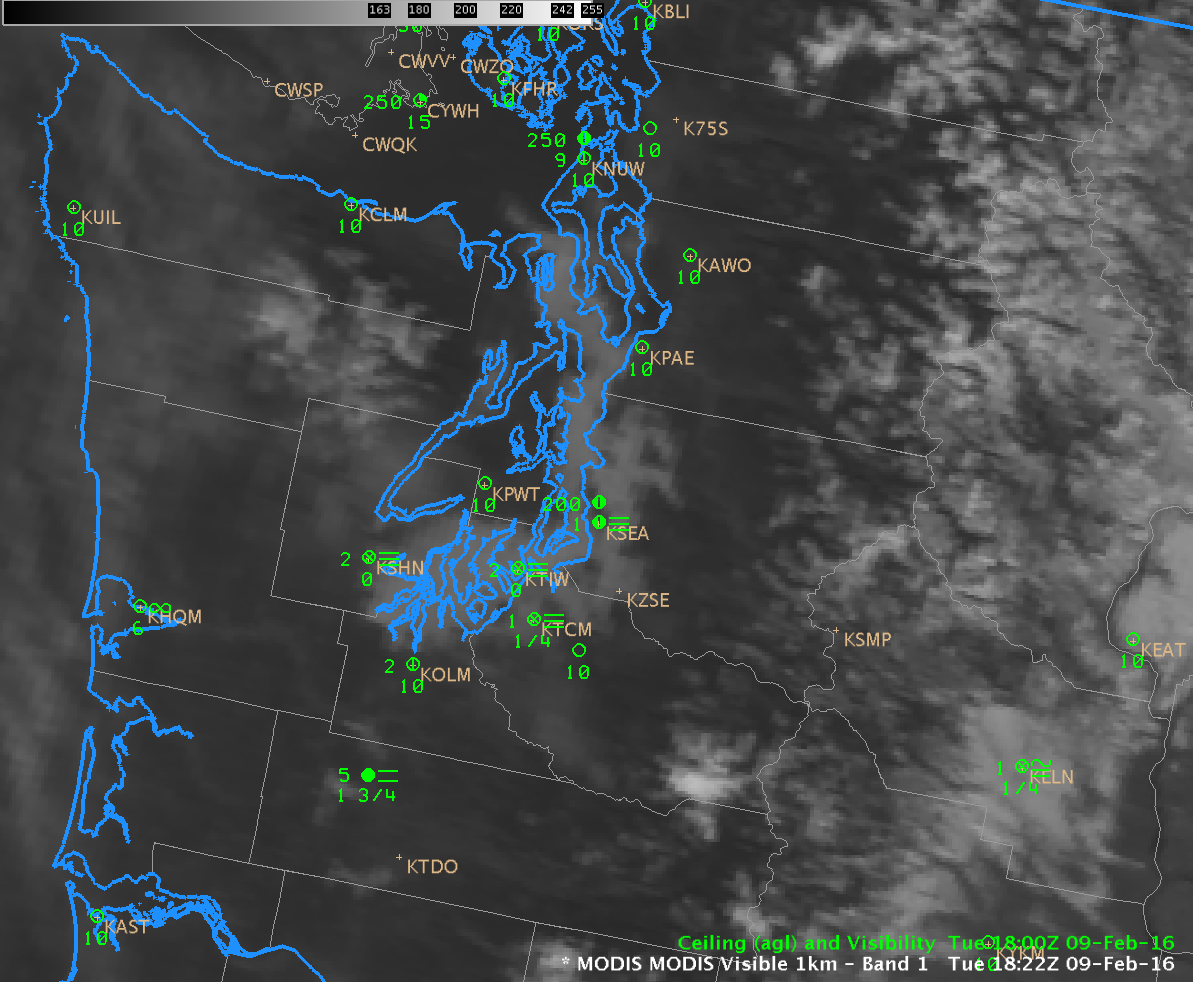
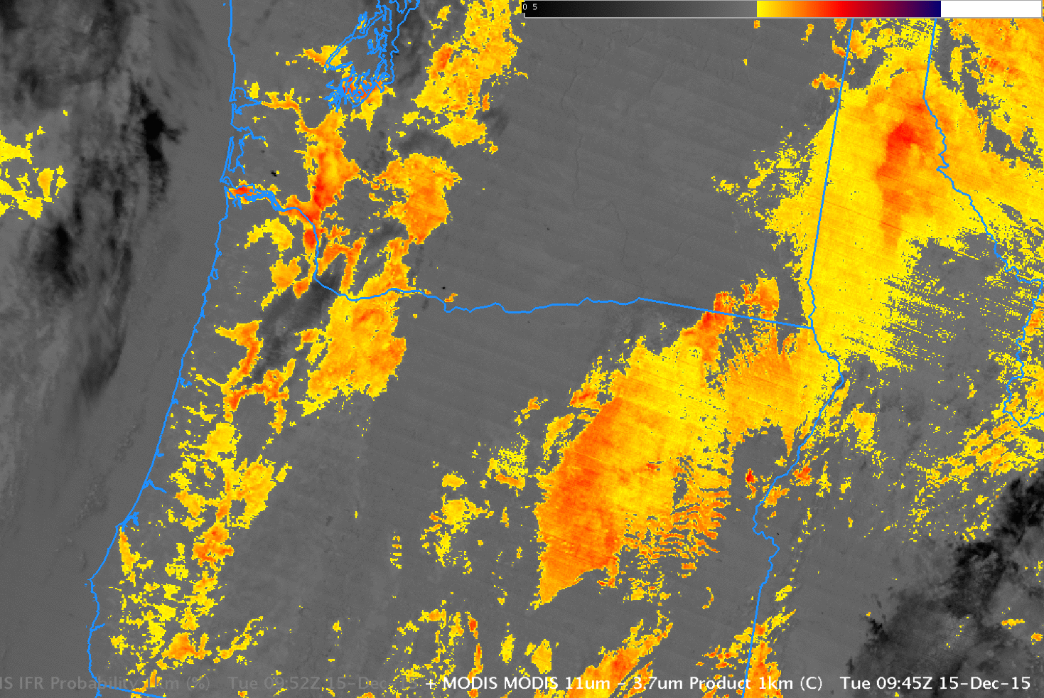
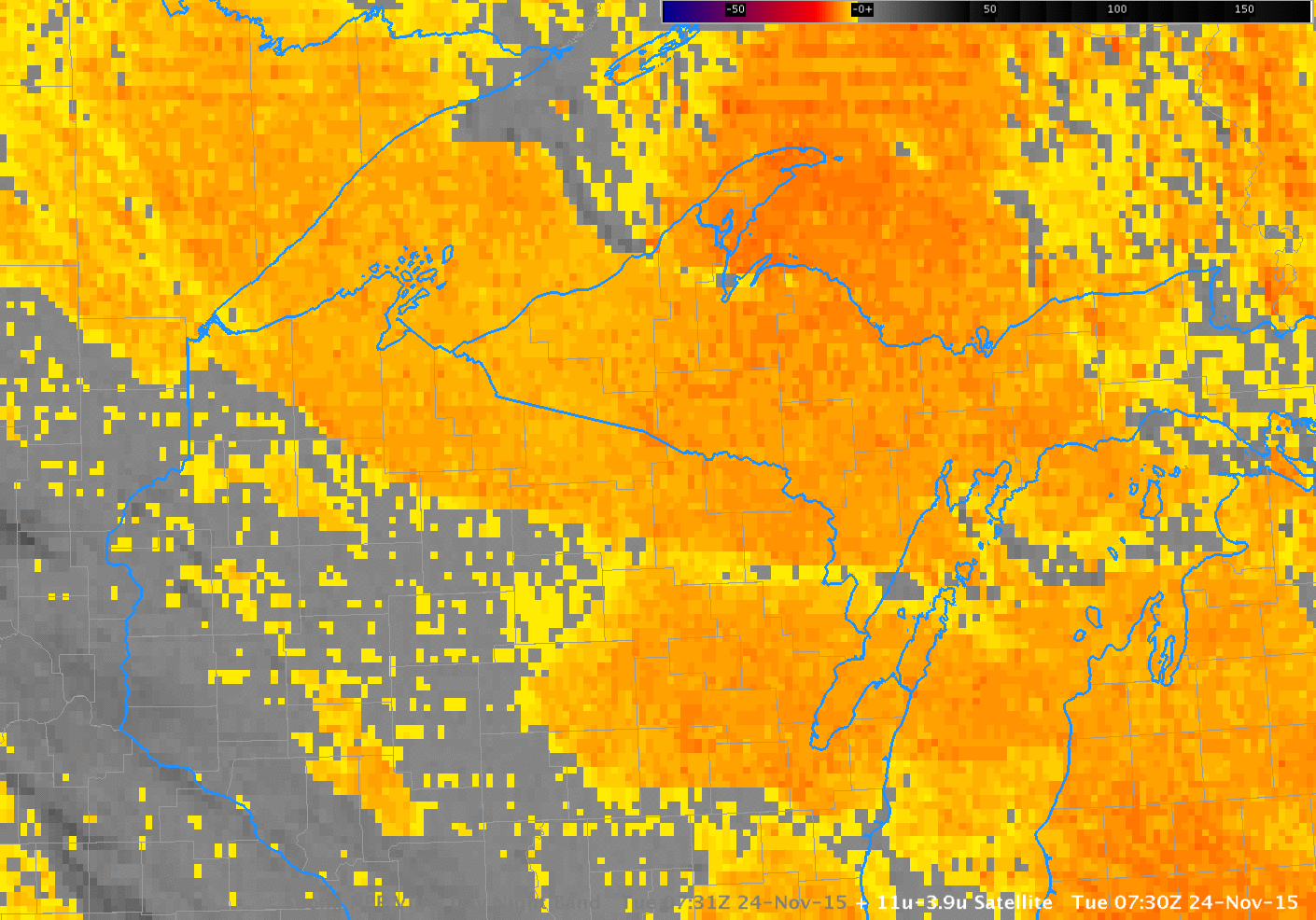
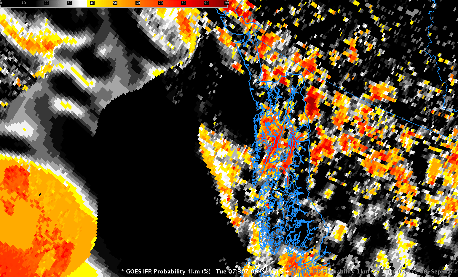
For a small-scale event, the nominal 4-km pixel size on GOES-15 and GOES-13 (a size that is closer to 6-7 km over Oregon because of the distance from the sub-satellite point) may prevent satellite detection of developing fog. The toggle below shows Brightness Temperature Difference fields at 0928 UTC from MODIS on Aqua, as well as the GOES-R IFR Probability fields computed using the MODIS data.  As with GOES data, the presence of cirrus in the Brightness Temperature Difference field is obvious and shown by a black enhancement.  Little signal is present over Baker County.  (There is a strong signal, however, in the valleys of northwest Montana and northern Idaho — compare this to the GOES-based brightness temperature difference above).

Note:  MODIS resolution is 1-km;  data from the Advanced Baseline Imager (ABI) on GOES-R will have nominal 2-km resolution at the sub-satellite point.

modis_btd_ifr_10nov_0928toggle

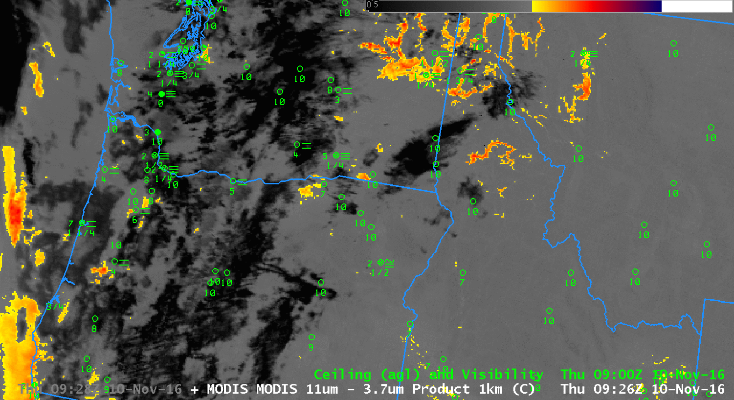
MODIS Brightness Temperature Difference fields (3.7 µm – 11 µm) and MODIS-based GOES-R IFR Probability, 0928 UTC on 10 November 2016 (Click to enlarge)

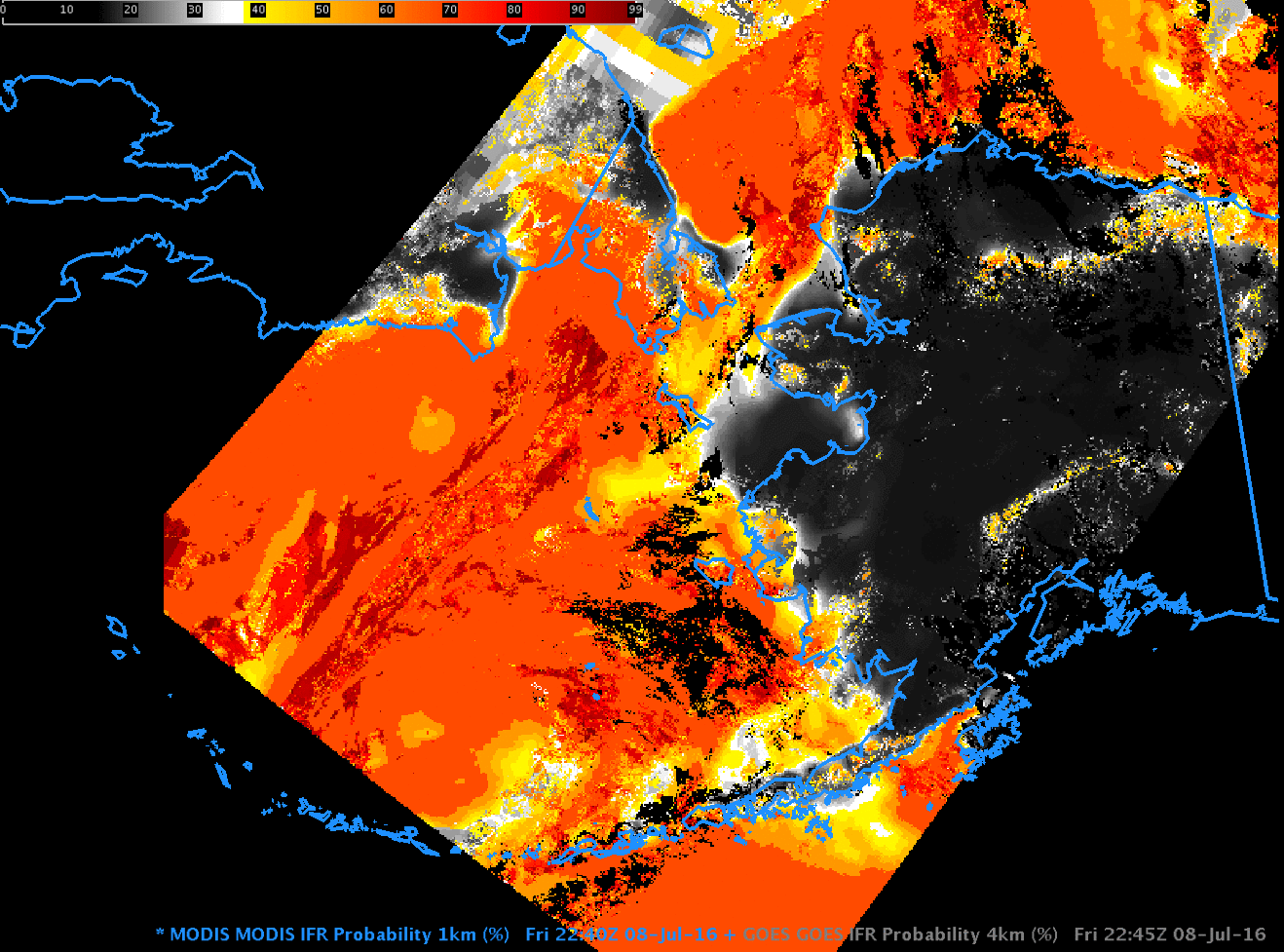
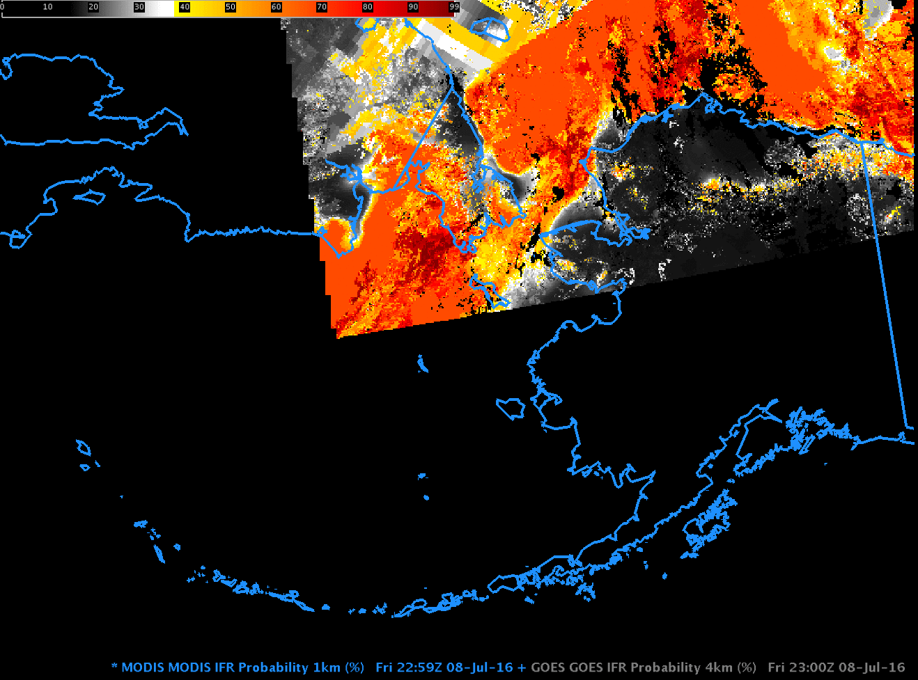
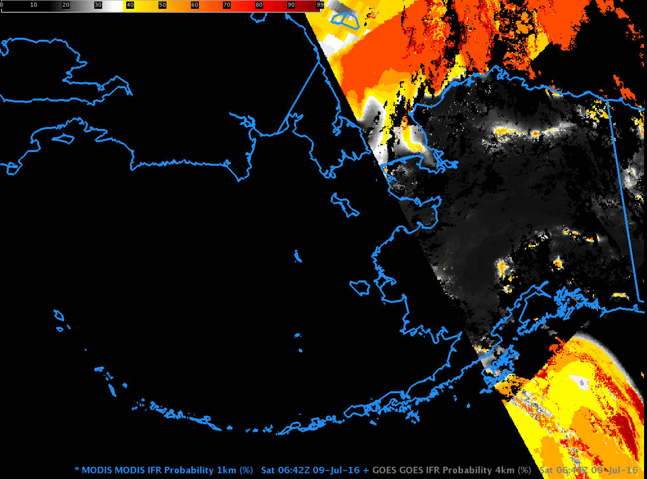
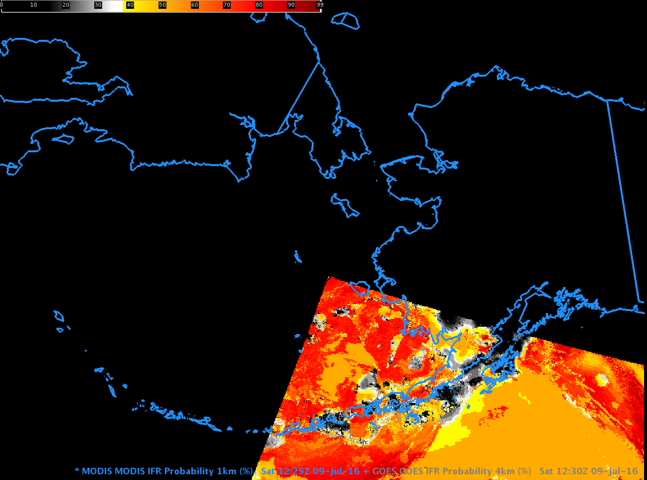
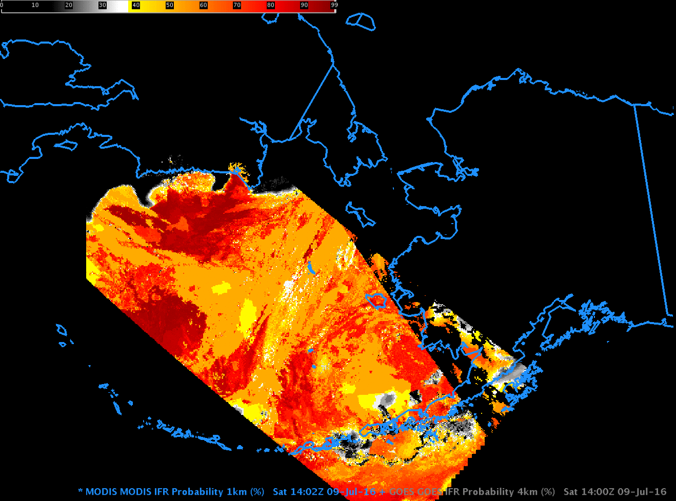
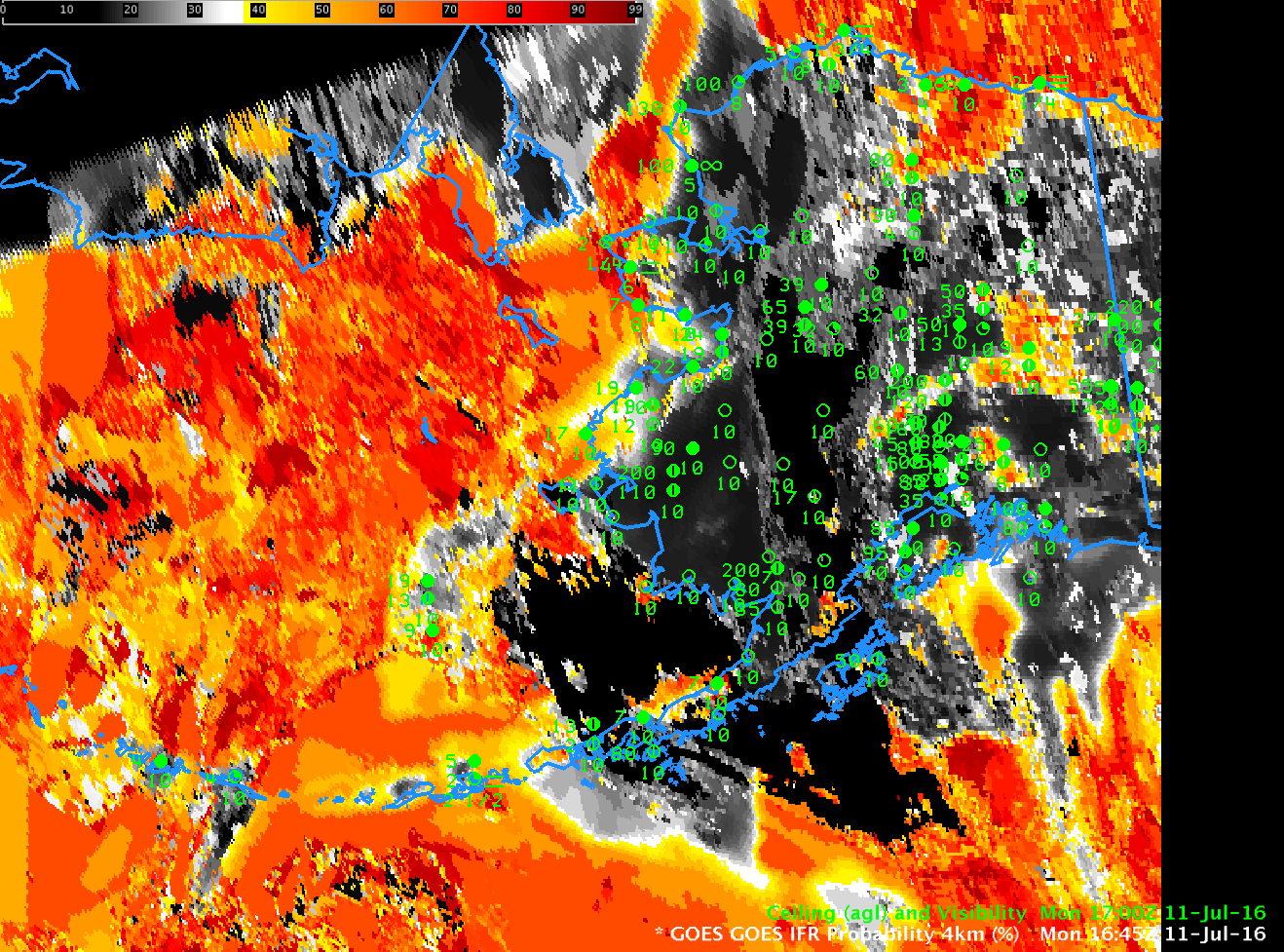
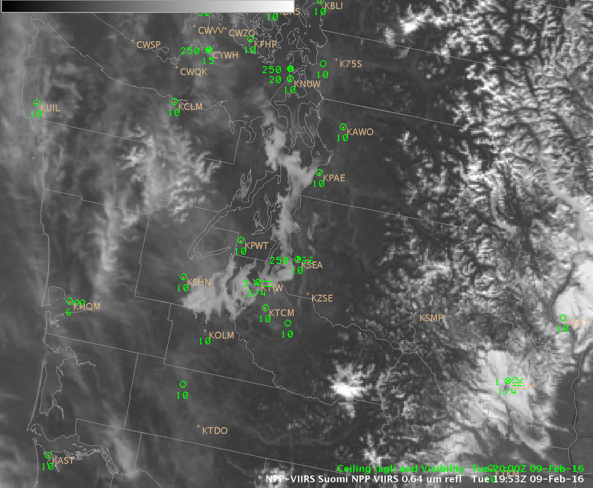
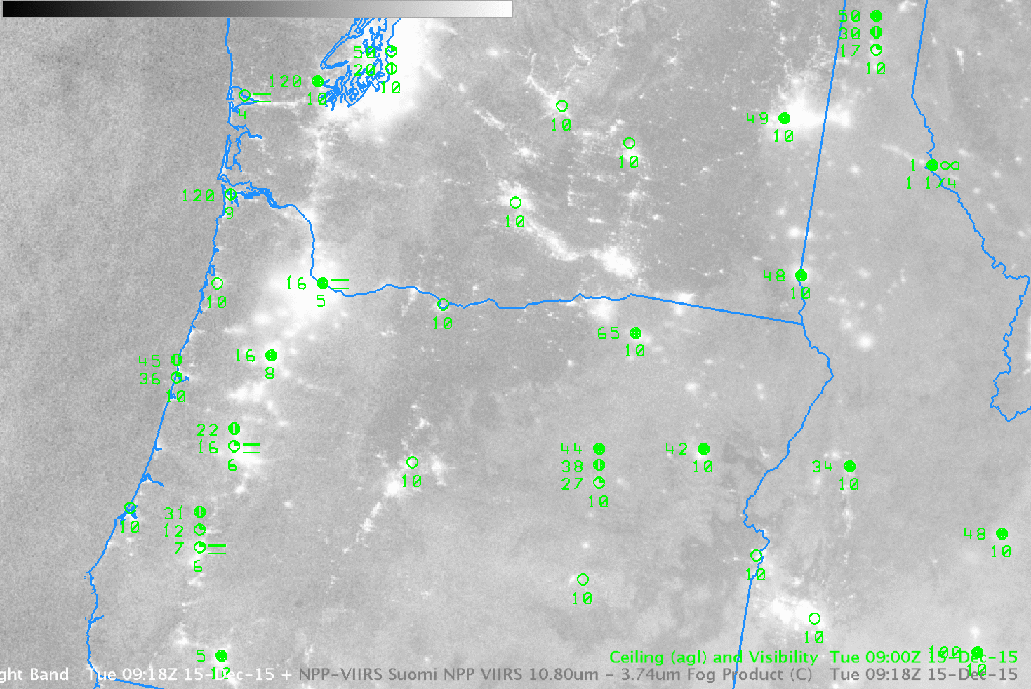
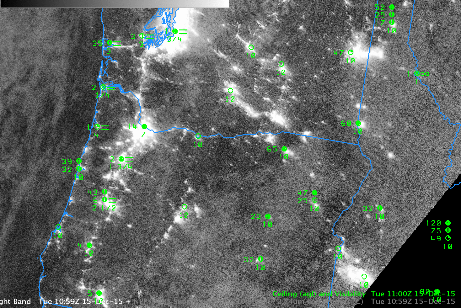
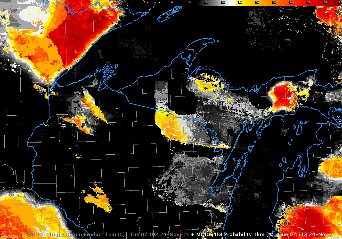
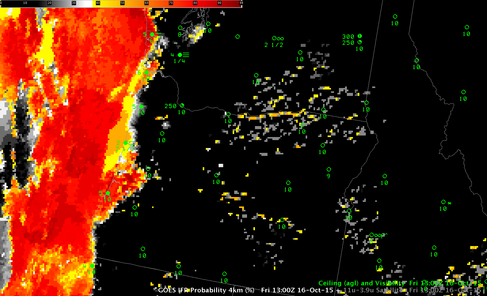
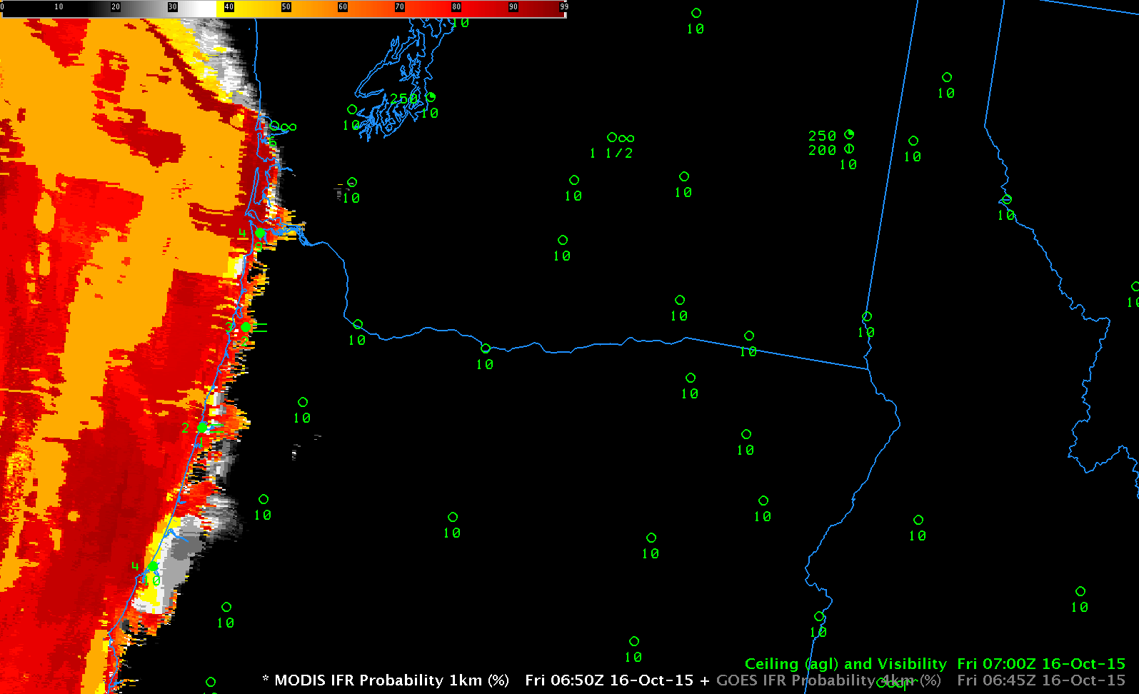
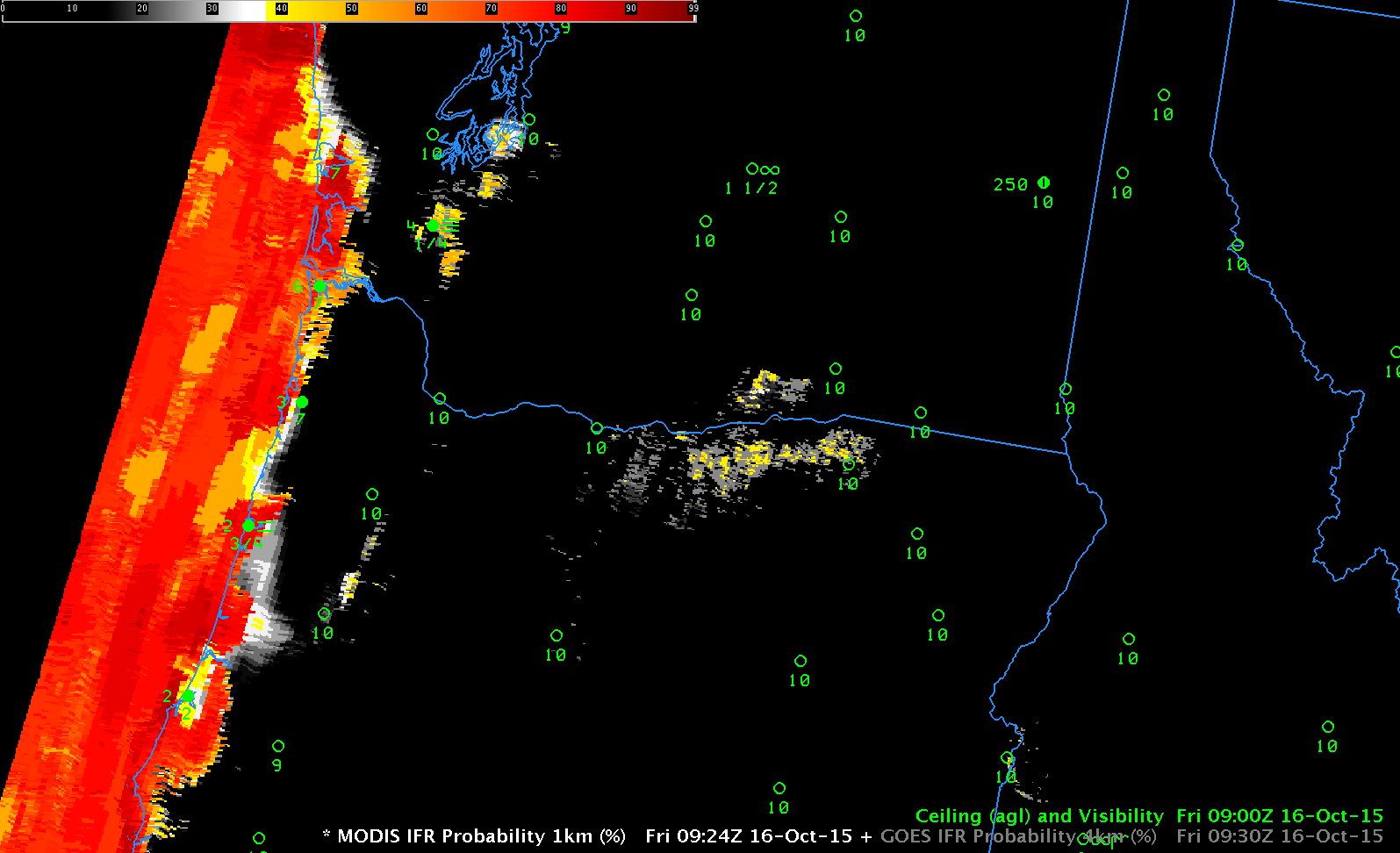
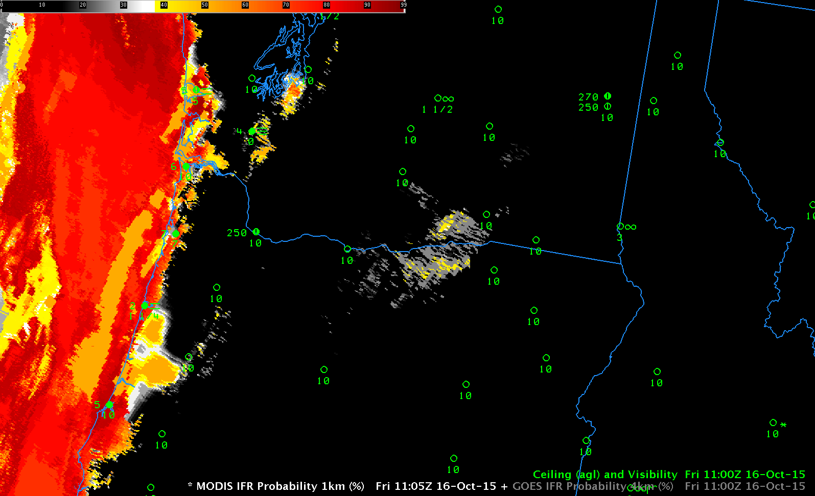
What does the GOES-based GOES-R IFR Probability field show during the early morning hours of 10 November? The animation below, from 0800-1200 UTC, shows some returns in/around Baker County. It would have been difficult to use this product alone to diagnose this fog feature however. (It did do a better job of diagnosing the presence of fog over northwest Montana and western Oregon where Advisories were later issued).

goesr_ifr_10nov_0800_1200anim

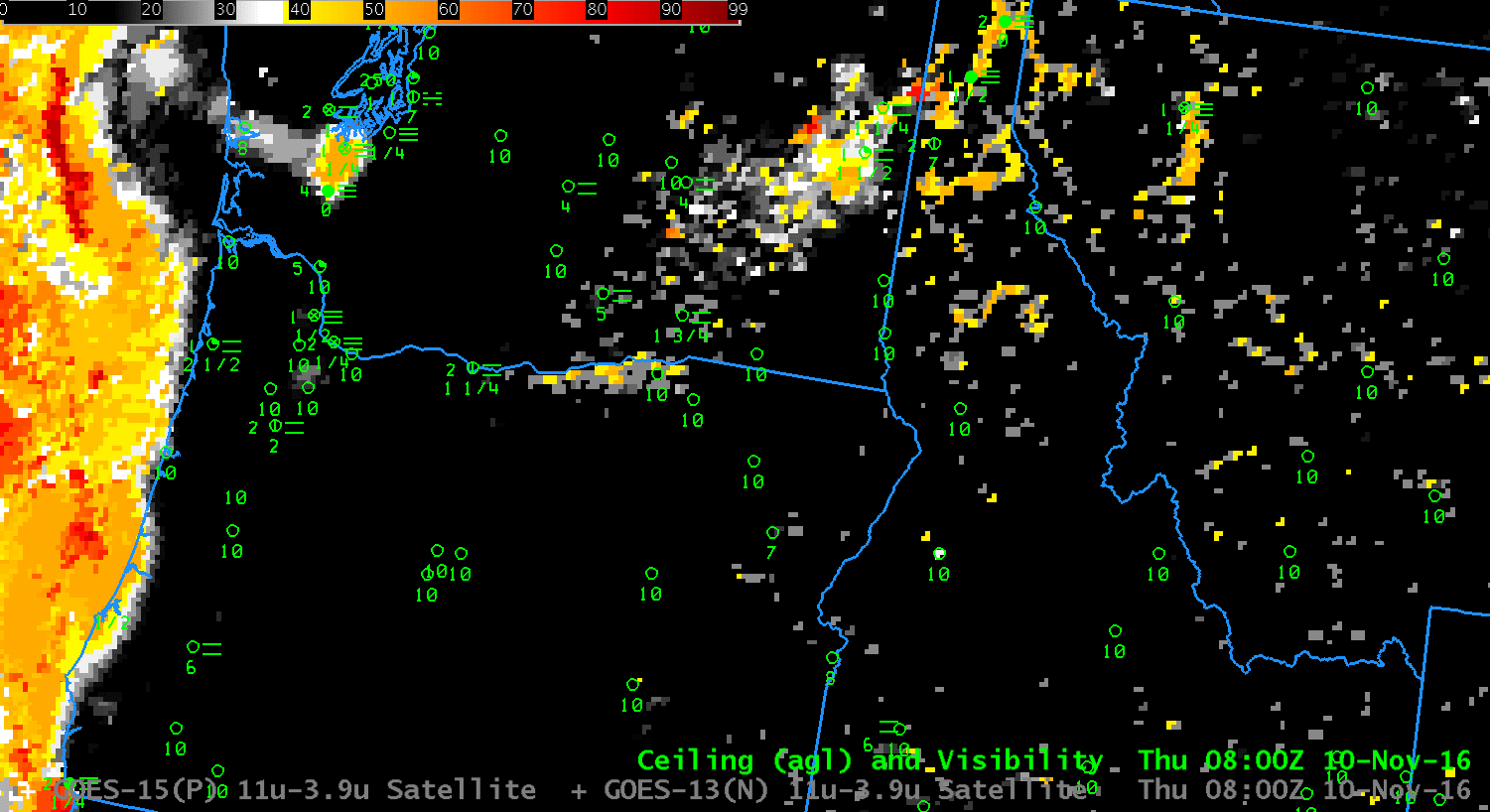
GOES-R IFR Probability fields, hourly from 0800 – 1200 UTC on 10 November 2016 (Click to enlarge)

MODIS and GOES IFR Probabilities over Alaska

GOES-R IFR Probabilities computed using GOES-15 pixels over Alaska suffer from problems inherent in any Geostationary Data Product at high latitudes: Pixel sizes are large. In addition, ‘limb brightening’ — that is, the shift in a brightness temperature towards cooler values because the path length of photon towards the satellite travels through more of the upper (colder) troposphere (a cooling that is also dependent on wavelength being sensed) — affects the brightness temperature difference product that is used to detect water-based clouds. MODIS data from Terra and Aqua has a much higher spatial resolution and a superior view angle. It’s fairly simple to use both MODIS data to get an idea of conditions in and around Alaska, and then use GOES data to approximate the temporal change. Terra and Aqua view Alaska frequently (link) — it’s uncommon to go more than 6 hours without a view.

The toggles below show a series of MODIS IFR Probabilities and corresponding GOES-15 IFR Probabilities from late on 8 July 2016 through mid-day on 9 July 2016. From 2100 UTC to 1400 UTC — 17 hours — there are 7 separate MODIS views of Alaska, and they show similar features. For example, the high terrain of the Brooks Range is apparent: larger values of IFR Probabilities are noted there. The same is true over south central Alaska, over the Alaska Range in between Anchorage and Fairbanks. Interpretation of IFR Probability fields over the State require this background knowledge of Topography.

MODIS_GOES_IFR_2100_08July2016toggle

MODIS-based and GOES-15-based GOES-R IFR Probability fields, 2100 UTC on 8 July 2016 (Click to enlarge)

MODIS_GOES_IFR_2245_08July2016toggle

MODIS-based and GOES-15-based GOES-R IFR Probability fields, 2245 UTC on 8 July 2016 (Click to enlarge)

MODIS_GOES_IFR_2300_08July2016toggle

MODIS-based and GOES-15-based GOES-R IFR Probability fields, 2300 UTC on 8 July 2016 (Click to enlarge)

MODIS_GOES_IFR_0645_09July2016toggle

MODIS-based and GOES-15-based GOES-R IFR Probability fields, 0645 UTC on 9 July 2016 (Click to enlarge)

MODIS_GOES_IFR_0815_09July2016toggle

MODIS-based and GOES-15-based GOES-R IFR Probability fields, 0815 UTC on 9 July 2016 (Click to enlarge)

MODIS_GOES_IFR_1230_09July2016toggle

MODIS-based and GOES-15-based GOES-R IFR Probability fields, 1230 UTC on 9 July 2016 (Click to enlarge)

MODIS_GOES_IFR_1400_09July2016toggle

MODIS-based and GOES-15-based GOES-R IFR Probability fields, 1400 UTC on 9 July 2016 (Click to enlarge)

The scenes above suggest that most IFR Conditions near Alaska are offshore during the early morning of 9 July. On 11 July 2016, some of those regions of reduced visibility crept onshore, as shown in the plot below from this site, where surface stations are color-coded by Flight Rules: Red and Magenta denote IFR and Low IFR conditions.

METARS_1700_11July2016

Surface METARS, 1700 UTC on 11 July 2016 (Click to enlarge)

GOES-15-based IFR Probability fields from near that time show high probabilities along the coastline of Alaska.  Note that the presence of IFR Conditions can also be deduced from this set of webcams! Consider, for example, this webcam site just west of Prudhoe Bay, in a region where GOES-based IFR Probabilities are high.

GOES_IFR_1700_11July2016

GOES-15-based GOES-R IFR probability fields, 1700 UTC on 11 July 2016, along with surface observations of ceilings and visibilities (Click to enlarge)

Fog over the Tennessee River Valley

IFRP_0115_1315stepanim_17Feb2016

GOES-R IFR Probability fields, every two hours from 0115 through 1315 UTC on 17 February 2016 (Click to enlarge)

GOES-R IFR Probability fields showed large values over parts of Kentucky and Tennessee during the overnight hours on 16-17 February 2016, as shown in the animation above (every 2 hours from 0115 through 1315 UTC). (IFR or near-IFR Conditions were present over the region of enhanced IFR Probabilities) For much of the overnight hours, mid-level and high clouds prevented an unobstructed satellite view of low clouds, so Rapid Refresh model output was the principle driver in IFR Probabilities. When that happens, the character of the IFR Probability field is less pixelated (it’s a flatter field) and values are smaller. At the end of the animation — 1315 UTC — satellite observations of low clouds have improved and the GOES-R IFR Probability field is (1) more pixelated, as expected when satellite data are used and (2) showing higher values because Satellite Predictors can be used in the computation of IFR Probability.

MODIS data from Terra and Aqua satellites can also be used to compute IFR Probability fields, and the high spatial resolution of the MODIS instrument (1-km vs. nominal 4-km on GOES) can yield superior results for valley fogs, for example (The effects of some rivers are apparent in the 0354 UTC image over western Tennessee, for example). For a large-scale event as above, however, GOES-based resolutions can be adequate. The toggle of MODIS-based GOES-R IFR Probabilities at 0354 UTC and 0810 UTC is shown below. Patchy clouds (that prevent MODIS from viewing low clouds) are more apparent in the 0354 UTC image than in the 0810 UTC image.

MODIS_IFRP_0354_0810UTC_17Feb2016toggle

MODIS-based GOES-R IFR Probabilities, 0354 and 0810 UTC on 17 February 2016 (Click to enlarge)

Suomi NPP Overflew the Tennessee River valley just after midnight local time, and the toggle of the Day Night band and the Brightness Temperature Difference field (11.45 – 3.74) is shown below. Extensive cloud cover is apparent. The importance of the IFR Probability fields is that it incorporates surface information (from the Rapid Refresh predictions of saturation in the lowest 1000 feet of the model atmosphere) so that fog and low stratus that impacts transportation by reducing visibilities can be distinguished from mid-level stratus that has a smaller impact.

SNPP_DNB_BTD_0735UTC_17Feb2016toggle

Suomi NPP Brightness Temperature Difference fields (10.8 µm – 3.74 µm) and Day Night band visible imagery (0.70 µm) at 0735 UTC on 17 Feburary 2016 (Click to enlarge)

Small-scale Fog Event near Puget Sound

IFRProbability_9Feb_11_22UTCanim

GOES-R IFR Probabilities computed with GOES-15 and Rapid Refresh Data, 1100-2200 UTC on 9 February 2016 (Click to enlarge)

GOES-R IFR probabilities on Tuesday 9 February captured the development of a small-scale fog event in/around the southern part of Puget Sound in Washington State. The animation above shows high IFR Probabilities developing shortly before sunrise and persisting through most of the day in a region including Shelton, Olympia, Tacoma and Seattle.

MODIS visible data, below, from the Terra Satellite overpass shortly after 1800 UTC, below, shows the fogbank over the most of Puget Sound, extending inland only over the southern part of the sound.

MODISVIS_1822

MODIS Visible Imagery (0.65 µm), 1822 UTC on 9 February (Click to enlarge)

Suomi NPP viewed Puget Sound on two consecutive overpasses on 9 February, and visible imagery from those passes, just before 2000 UTC and near 2130 UTC, are shown below.  Fog Dissipation is apparent in the later image, which is consistent with the animation of IFR Probability at the top of this post, which animation shows IFR Probabilities declining in value after 2100 UTC.

SNPPVIS_1953_2122step

Suomi NPP Visible Imagery (0.64 µm), 1953 and 2122 UTC on 9 February (Click to enlarge)

Dense Fog Advisories in southern Idaho

Dense Fog Advisories were issued over southern Idaho early on 19 January 2016. GOES-R IFR Probability fields, below, show high probabilities in this region. Surface observations are not common over northern Utah/southern Idaho, and the hourly animation does show IFR Conditions observed near the high IFR Probabilities over southern Idaho and northern Utah (Logan, UT — KLGU — at 41:47 N, 111:51 W, in far northern Utah from 0300 – 1300 UTC; Elko NV — KEKO — at 40:50 N, 115:47 W also shows IFR conditions).  The Snake River Valley in Idaho also shows high IFR Probabilities during parts of the animation.

GOES-R IFR Probability fields fuse together information from GOES-15 (or, in the eastern part of the USA, GOES-13) and Rapid Refresh Data. Highest probabilities occur where the satellite detects low (water-based) clouds and where the Rapid Refresh Model predicts low-level saturation. High IFR Probabilities don’t necessarily guarantee the presence of IFR Conditions — but they are a flag that should prompt a forecaster to be alert to the possibility that IFR conditions are present nearby or are developing. When dense fog is valley-based as might happen in the Rocky Mountains, GOES Pixel footprints and Rapid Refresh model resolution are sometimes too coarse to resolve completely the fog. MODIS data (bottom) has 1-km horizontal resolution and IFR Probabilities computed from MODIS data are more likely to resolve small valleys.

IFR_P_IdahoUtah_19January_anim_0200_1500

GOES-R IFR Probability fields computed from Rapid Refresh Model Output and GOES-15 Satellite Data, hourly from 0200 – 1500 UTC, 19 January 2016 (Click to enlarge)

MODISIFR_1023UTC_19Jan

GOES-R IFR Probability computed from MODIS data and Rapid Refresh Model output, 1023 UTC 19 January 2016 (Click to enlarge)

Fog vs. Stratus over the Pacific Northwest

Brightness Temperature Difference (10.7 µm – 3.9 µm) from GOES highlight regions of water-based clouds:  water-based clouds emit 10.7 µm radiation nearly as a blackbody does, but those clouds do not emit 3.9 µm radiation as a blackbody.  Thus, the brightness temperature computed from the radiation detected by the satellite (GOES-15 in this case) — a computation that assumes a blackbody emission — is relatively cooler for the 3.9 µm data compared to the 10.7 µm data.  A water-based cloud is normally stratus, and the pertinent question for aviation purposes (for example) is:  Is the ceiling of that cloud near the surface?  (That is:  Is the stratus also a fog bank, or is it “just” mid-level stratus?)

GOESIFRP_BTD_15December2015_0500UTCtoggle

GOES-15 Brightness Temperature Difference (10.7 µm – 3.9 µm) and GOES-based GOES-R IFR Probabilities, 0500 UTC 15 December 2015 (Click to enlarge)

The toggles above (0500 UTC) and below (0900 UTC) show how the GOES-R IFR Probability fields capably screen out many regions of mid-level stratus. This is achieved by fusing the brightness temperature difference information with data from the Rapid Refresh Model. If the lowest 1000 feet of the Rapid Refresh Model is not near saturation, probabilities of IFR conditions are reduced.

GOESIFRP_BTD_15December2015_0900UTCtoggle

As above, but at 0900 UTC 15 December 2015 (click to enlarge)

GOESIFRP_BTD_15December2015_1200UTCtoggle

As above, but at 1200 UTC 15 December 2015 (click to enlarge)

Toggles from 1200 UTC (above) and 1400 UTC (below) continue to show IFR Conditions mostly confined to regions near the Willamette Valley in eastern Oregon — banked up against the higher terrain to the east of the Willamette, and also over the higher terrain of northeastern Oregon (Click here for a toggle between the 1400 UTC IFR Probability field and Topography). IFR Conditions are a function of ceilings above ground (not above Mean Sea Level), so it’s important to recognize the influence of topographic features on an IFR Probability field. Fog/Low stratus can bank up against a topographic feature, and/or it can shroud the top of a topographic feature.

Note also how at 1400 UTC high clouds have impinged upon extreme northwest Oregon and coastal western Washington. In these regions IFR conditions nevertheless persist under the high clouds, but satellite data alone does not indicate low cloudiness. In this region, the inclusion of Rapid Refresh data in the GOES-R IFR Probability algorithm allows the IFR Probability field to continue to provide useful information about the presence of fog/low stratus.

GOESIFRP_BTD_15December2015_1400UTCtoggle

As above, but at 1400 UTC 15 December 2015 (click to enlarge)

MODIS and Suomi NPP afforded high-resolution images of the fog/stratus banks over the Pacific Northwest on 15 December. The brightness temperature difference fields and MODIS-based IFR Probability fields from MODIS at 0533 and 0945 UTC, below, support the observations from the coarser-resolution GOES fields above.

MODISIFRP_BTD_15December2015_0533UTCtoggle

As above, but for MODIS data at 0533 UTC 15 December 2015 (click to enlarge)

MODISIFRP_BTD_15December2015_0945UTCtoggle

As above, but for MODIS data at 0945 UTC 15 December 2015 (click to enlarge)

GOES-R IFR Probability fields are not yet computed using data from the Suomi NPP Satellite, but the Day Night band and the Brightness Temperature Difference field give information about the presence of cloudiness. For the case of Suomi NPP data, however, it’s more important to consider surface-based observations to confirm regions of low clouds/fog or mid-level stratus. Note also that December 15 was shortly after a New Moon, and the crescent moon that could give illumination was below the horizon (that is, it had set) at 0918 and 1059 UTC.

Note that Suomi NPP Near-Constant Contrast Day Night Band imagery was scheduled to start flowing in to AWIPS II on 14 December 2015 via the SBN. It should be available in NWS offices now.

SNPPBTD_DNB_15December2015_0918UTCtoggle

Suomi NPP Day Night Band Visible Imagery (0.70 µm) and Brightness Temperature Difference (10.35 µm – 3.74 µm), 0918 UTC 15 December 2015 (Click to enlarge)

SNPPBTD_DNB_15December2015_1059UTCtoggle

Suomi NPP Day Night Band Visible Imagery (0.70 µm) and Brightness Temperature Difference (10.35 µm – 3.74 µm), 1059 UTC 15 December 2015 (Click to enlarge)

Are IFR Conditions Present?

SNPP_BTD_DNB_0731_24Nov2015toggle

Suomi NPP Visible (0.70 µm) Day Night Band Imagery and Infrared Brightness Temperature Differences (11.45 µm – 3.74 µm), 0731 UTC on 24 November 2015 (Click to enlarge)

Low clouds (with a sharp southern edge) were over northern Wisconsin during the early morning of 24 November 2015. Are IFR Conditions present? Can you tell from the satellite imagery alone? The cloud bank stretched over northern Wisconsin seems thick compared to the bank of clouds over northeastern Wisconsin (centered on southern Green Bay). The city lights of Duluth are not visible in the same way that the city lights of Green Bay are in the Day Night band imagery. Clouds in general are distinct with the near-full moon providing ample illumination.

Both GOES and MODIS Brightness Temperature Difference fields, below, show a signal consistent with low clouds over most of northern WI and adjacent regions.  But are there IFR Conditions?

GOES_MODS_BTD_0749_24Nov2015toggle

GOES-13 Brightness Temperature Difference (10.7 µm – 3.9 µm) Fields (0730 UTC) and MODIS Brightness Difference Fields (11 µm – 3.9 µm) (0749 UTC)

IFR Probability fields blend the information available from satellite (are water-based clouds present?) with model output to yield a refined diagnostic of IFR Conditions. If there is saturation in the lowest levels (the lowest 1000 feet) of the model, then Probabilities of IFR Conditions are increased. If the lowest levels of the model are relatively dry, in contrast, then IFR Probabilities are reduced. On the morning of 24 November, the latter condition occurred over northern Wisconsin. IFR Probabilities computed from MODIS and GOES-13 satellite values are shown below. Probabilities are very low over most of Wisconsin where mid-level stratus (with varying bases) was present: IFR conditions were not generally observed in the regions where water-based clouds were indicated by the satellite. Mid-level stratus can look, from the top, very similar to fog, but it’s impossible for the satellite alone to discern what’s happening at the cloud base. Model data helps the IFR Probability algorithm screen out regions where mid-level stratus is occurring.

MODS_GOES_IFR_OBS_0731_24Nov2015toggle

MODIS-based GOES-R IFR Probabilities (0751 UTC), GOES-13-based GOES-R IFR Probabilities (0731 UTC), and GOES-based GOES-R IFR Probabilities with surface observations of ceilings and visibilities (Click to enlarge)

Resolution Benefits from MODIS

GOES_IFR_16Oct_0200_1400step2hour

GOES-R IFR Probability fields, every 2 hours from 0200 through 1400 UTC on 16 October 2015 (Click to enlarge)

The GOES-R IFR Probability fields over Oregon and Washington on the morning of 16 October 2015 correctly diagnose low ceilings and reduced visibilities along the coast, even when high clouds intervene at the end of the animation above (especially evident at 1300 UTC, below). In addition to marine stratus that is reducing visibility/ceilings along the coast, surface observations suggest a valley fog is forming in/around Centralia/Chehalis Washington (KCLS). However, GOES-based IFR Probability fields do not become enhanced in that area. Why not?

GOES_IFR_16Oct_1300

GOES-R IFR Probability computed from GOES-15, 1300 UTC on 16 October 2015. Note the Character of the field near Newport OR (KONP); the uniformity of the field is characteristic of regions where satellite signals cannot be used because of high clouds (Click to enlarge)

The valley of the Chehalis River, in which the fog is forming, is far too narrow to be resolved by GOES-15, which satellite has 4-km pixel sizes at the sub-satellite point. (Pixels are closer to 6 km in size over southern Washington). Higher-resolution MODIS data (with a 1-km pixel size) can be used to create GOES-R IFR Probabilities, and MODIS overpasses viewed Centralia/Chehalis at 0650, 0924 and 1105 UTC. The imagery below toggles between MODIS-based and GOES-based GOES-R IFR Probabilities at those times.  Even as early as 0645 UTC, the MODIS-based IFR Probability fields are suggesting that a fog is starting to develop.  At later times the MODIS-based IFR Probability values are much larger than the GOES-based values.  MODIS data can give an early alert to the development of small-scale fog.

MODIS_GOESIFR_PROB_16Oct_0650toggle

MODIS-based (0650 UTC) and GOES-15-based (0645 UTC) GOES-R IFR Probability fields (Click to enlarge)

MODIS_GOESIFR_PROB_16Oct_0924toggle

MODIS-based (0924 UTC) and GOES-15-based (0930 UTC) GOES-R IFR Probability fields (Click to enlarge)

MODIS_GOESIFR_PROB_16Oct_1105toggle

MODIS-based (1105 UTC) and GOES-15-based (1100 UTC) GOES-R IFR Probability fields (Click to enlarge)

MODIS resolution versus GOES resolution

WV_MODIS_GOES_IFRPROB_0315_11Sep2015toggle

MODIS-based (0300 UTC) and GOES-based (0315) UTC GOES-R IFR Probability fields on 11 September 2015 (Click to enlarge)

MODIS data (from Terra and Aqua) and GOES data can both be used to create GOES-R IFR Probability fields. The differences between the two data sources — especially spatial resolution — are obvious in the toggle above. MODIS data can capture the development of fingers of fog that develop in small river valleys, and GOES data cannot (although, of course, a forecaster with knowledge of the topography might appropriately tailor a forecast). In the toggle above, MODIS data capture the small tributaries of the Ohio River in Ohio and West Virginia that likely contain fog at 0300 UTC (11 PM local time). GOES data smear out that information. This is true later at night as well, below, at 0715 UTC. River valleys show higher IFR Probabilities than adjacent mountains. Valley fog is easier to delineate with MODIS data than with GOES data.

WV_MODIS_GOES_IFRPROB_0715_11Sep2015toggle

MODIS-based (0715 UTC) and GOES-based (0715) UTC GOES-R IFR Probability fields on 11 September 2015 (Click to enlarge)

GOES-R IFR Probabilities at High Latitudes

AK_DenseFog_8Sep2015

Screenshot from the Juneau, AK WFO on 8 September 2015. The yellow region has a Dense Fog Advisory (Click to enlarge)

A challenge in using GOES-R IFR Probabilities at high latitudes is that GOES pixels are larger, typically twice or three times the size of pixels over the lower 48. If Fog is starting out as a small-scale phenomenon, the early development of the feature can be missed. Dense fog developed over southeast Alaska on the morning of 8 September. The animation of GOES-15-based IFR Probabilities, below, shows the slow increase in areal extent to the IFR Probabilities in the six hours between 0445 and 1045 UTC; values also increased.  This slow increase in concert with observations can increase confidence that wide-spread dense fog is possible.

AK_GOES_IFRPROB_0445_1045UTC_08Sept2015stepanim

GOES-15 based GOES-R IFR Probabilities, 0445, 0715 and 1045 UTC on 8 September 2015 (Click to enlarge)

MODIS data from Terra and Aqua can also be used to compute IFR Probabilities, and the high resolution information from these two polar orbiting satellites can clarify where fog might be occurring. Additionally, MODIS fields are a bit more frequent over Alaska than they are over the lower 48. The 0600 and 0737 UTC passes, shown below, show how MODIS data can be used to refine the GOES-based information at times during the night. The temporal change between MODIS information at 0600 and 0737 UTC also confirms the trend observed in GOES data alone.

AK_GOES_MODIS_IFRPROB_0600UTC_08Sept2015toggle

GOES-15 and MODIS-based GOES-R IFR Probabilities, 0600 UTC 8 September 2015 (Click to enlarge)

AK_GOES_MODIS_IFRPROB_0730UTC_08Sept2015toggle

GOES-15 and MODIS-based GOES-R IFR Probabilities, ~0730 UTC 8 September 2015 (Click to enlarge)