Category Archives: Day/Night Band

Fog near Hanford California

Tweeted Message from the National Weather Service in HNX (Hanford, CA) showing GOES-R IFR Probabilities in the central Valley of California (click to enlarge)

The National Weather Service in Hanford tweeted the image, above, of IFR Probability this morning. How did the evolution of IFR Probabilities compare to that of brightness temperature difference fields?

The hourly animation, below, suggests that data from the Rapid Refresh model was likely crucial in determining exactly where the lowest visibility occurred; the brightness temperature difference field did not capture the horizontal extent of the narrow band of fog that developed to the east of Interstate 5 (The interstate is the purple line in the animation). Indeed, the brightness temperature difference field appears to offer little in the way of forecast value, and differences trend to zero as the sun starts to rise at the end of the animation. In contrast, both IFR and LIFR Probabilities have peak values where ceilings are obscured and visibilities are near zero, in and around Hanford, and those large values persist through sunrise.

Hourly GOES-R IFR Probabilities (Upper Left, computed with data from GOES-15) with ceilings and visibilities plotted, Hourly GOES-R LIFR Probabilities computed with data from GOES-15 (Lower Left), GOES-15 Brightness Temperature Difference (10.7µm – 3.9µm) (Upper Right), Suomi NPP Day Night Band and Brightness Temperature Difference (11.45µm – 3.74µm) (Lower Right), times as indicated (Click to enlarge)

Suomi NPP overflew the central Valley at 0938 UTC. The Day Night Band and the brightness temperature difference (11.45µm – 3.74µm) field, below, do not contain signatures of dense fog near Hanford.

As above, but at 0945 UTC, when Suomi NPP data were present (Click to enlarge)

The two-hour time-lapse video, below, shows the evolution of the Fog at the National Weather Service Office in Hanford on the morning of 4 November.

Successive Suomi NPP Scans Show Stratus/Fog movement

Suomi NPP Day/Night Band at 0926 and 1106 UTC on 9 October 2014 (Click to enlarge)

(A Blog post on Suomi NPP Imagery over the western US from 10 October is available here).

Polar orbiters typically don’t give good temporal resolution, especially near the Equator. In mid-latitudes, however, Polar Geometry can yield views over a wide area on two successive scans. This happened along the West Coast early in the morning on 9 October. Two regions show noticeable changes in stratus between the two times: stratus/fog extends farther down the Salinas Valley at the southern edge of image, and stratus/fog expands over southwestern Puget Sound in Washington. The Brightness Temperature Difference field (11.35µm – 3.74µm) from Suomi NPP for the same times shows a similar evolution over the Salinas Valley, but the view of Washington is obscured by thin cirrus. These cirrus (that show up as black enhancements below) are mostly transparent in the Day Night Band but not in the infrared bands.

Suomi NPP Brightness Temperature Difference (11.35µm – 3.74µm) at 0926 and 1106 UTC on 9 October 2014 (Click to enlarge)

MODIS instruments onboard Terra and Aqua yield spectral data that can be used to generate GOES-R IFR Probability Fields. The animation below shows high-resolution imagery of where IFR Probabilities are highest, but only at three distinct times: 2152 UTC on 8 October and 0537 and 0949 UTC on 9 October. An increase in IFR Probabilities around Monterey Bay is apparent (and consistent with the Suomi NPP Observations above); IFR Probabilities also increase along the Oregon Coast and around Puget Sound.

MODIS-based GOES-R IFR Probabilities at 2152 UTC 8 October, 0547 UTC 9 October and 0949 UTC 9 October (Click to enlarge)

How do GOES-based observations complement the Polar Orbiter data above?

GOES-15 based GOES-R IFR Probabilities, hourly from 0200 through 1400 UTC, 9 October 2014 (Click to enlarge)

The hourly animation above shows the slow increase of IFR Probability in/around Monterey Bay, and also a push of higher IFR Probability onto the Oregon Coast that occurs after the last MODIS-based IFR Image shown farther up. (Higher IFR Probabilities also spill into San Francisco Bay). Do surface observations of ceilings and visibilities agree with the IFR Probability fields? The loops below, from Oregon (below) and Monterey Bay (bottom) suggest that they do. For example, Eugene OR (and stations north and south of Eugene) show IFR conditions as the high IFR Probability field moves in after 1100 UTC. GOES-based data is valuable in monitoring the motion of IFR Probability fields; keep in mind, though, that small-scale features may be lost. For example, it is difficult for GOES to resolve the Salinas Valley.

GOES-15 based GOES-R IFR Probabilities, hourly from 0200 through 1500 UTC, 9 October 2014, with surface and ceiling observations superimposed (Click to enlarge)

GOES-15 based GOES-R IFR Probabilities from 0400 through 1400 UTC, 9 October 2014, with surface and ceiling observations superimposed (Click to enlarge)

IFR Probability along the West Coast

MODIS data from Terra and Aqua, Suomi NPP data, and GOES-15 data yield different types of information that can be used to observe clouds in a region. Probabilities of IFR conditions — that is, what’s going on at cloud base, which is a part of the cloud the satellite cannot see — can be produced by combining satellite observations of cloud tops and data from a model (such as the Rapid Refresh) that includes accurate predictions low-level moisture.

GOES-based IFR Probabilities (Upper Left), GOES-15 Brightness Temperature Difference (10.7µm – 3.9µm) (Upper Right), MODIS-based IFR Probabilities (Lower Right) at 0646 UTC, 0919 and 1058 UTC (Click to enlarge)

The three MODIS images, above (bottom right), show the slow encroachment of higher IFR Probabilities east-southeastward along the Sonoma/Marin county border. The high-resolution imagery from MODIS allows a more accurate depiction of the sharp edges that can occur as marine stratus penetrates inland around topographic features. MODIS data also suggests reduced ceilings in San Francisco.

As above, but at 0919 UTC only, with a toggle of MODIS Brightness Temperature Difference (11µm – 3.7 µm) and IFR Probability (Bottom Right) (Click to enlarge)

The 0919 UTC MODIS pass (from Aqua) happened to pass at a time when the GOES-West brightness temperature difference field was contaminated by stray light. The toggle above shows the difference between MODIS and GOES Brightness Temperature Difference fields at that time. MODIS is only detecting a signal where low clouds are present (or where soil differences allow the emissivitiy differences that can show up in the brightness temperature difference field, in this case over Nevada)

Suomi NPP overflew California at 1000 UTC, and those images are below. The brightness temperature difference field, and the Day Night band show clouds offshore, and city lights in and around San Francisco Bay and Monterey Bay. Regions of stratus have moved inland towards southern Sonoma County, over San Francisco, and over Monterey. There is a slight brightness temperature difference signal in the Suomi NPP data that extends down the Salinas Valley as well; it’s difficult to perceive cloudiness in the Day Night band in that region however.

As above, but with a toggle of Suomi NPP Brightness Temperature Difference and Day Night Band in the lower left, data at 1021 UTC (Click to enlarge)

The great strength of GOES data is its ability to monitor continuously the West Coast. Trends are therefore more easily observed. The hourly loop, below, shows that along much of the west coast, marine stratus stayed off shore through the night. Higher IFR Probabilities are also confined to regions where ceilings and visibilities were reduced. This is an improvement on the brightness temperature difference fields for the same time that have strong signals over much of the central Valley (for example, at 0500 and 1300 UTC, as well as at 0915 UTC, above).

GOES-15 IFR Probabilities, hourly from 0400 through 1300 UTC, 6 October 2014 (Click to enlarge)

Stratus and Fog over the northeast and mid-Atlantic States

GOES-13 Color-Enhanced Brightness Tempreature Difference Fields (10.7 µm – 3.9 µm), hourly from 0200 through 1100 UTC, 15 September 2014 (Click to enlarge)

Brightness Temperature Difference Fields from GOES-13 show large regions over Pennsylvania and surrounding states during the early morning hours of September 15th. (Note that the image at 0515 UTC, not in the loop above, shows the effect of stray light). If you look at the ceilings and visibilities in the imagery above, you will note that many regions where stratus/fog are indicated by the brightness temperature difference field (over upstate NY, for example), do not in fact show anything near IFR conditions. Always recall that the satellite is seeing the top of the cloud deck; whether or not that cloud extends to the surface is beyond the capability of present satellite systems. (You can infer it sometimes, of course, especially if the signal is confined to a narrow river valley, as occurs in the animation above: The Ohio River along the northern panhandle of West Virginia shows up very well).

GOES-13 IFR Probability Fields, hourly from 0200 through 1100 UTC, 15 September 2014 (Click to enlarge)

IFR Probability fields for the same time do a better job of highlighting only where reduced ceilings and visibilities are present. For example, the region of stratus over upstate New York is screened out, as well as the region over southern and southeastern Virginia. Probabilities are also quite high over the Ohio River Valley, where river fog is likely occurring. Note that IFR Probabilities over southwestern Indiana at the end of the animation have the characteristic look (a flat field) associated with IFR Probabilities created without the benefit of satellite data.

MODIS data were able to provide a a high-resolution image of this scene in the middle of the night. As with GOES, MODIS identified the large region of stratus over upstate New York and over southeastern Virginia, and the IFR Probabilities correctly screened out those stratus clouds. River Valleys show up distinctly along the Ohio River downriver from Pennsylvania; smaller IFR Probabilities surround the rivers. Sometimes MODIS data can give an early alert to the development of fog; in the present case, when MODIS overflew the region, fog development was at sufficiently large a scale that GOES-13 could also detect it.

MODIS Color-Enhanced Brightness Tempreature Difference Fields (11 µm – 3.9 µm) and IFR Probability Fields at 0722 UTC 15 September 2014 (Click to enlarge)

Suomi NPP data also viewed the developing river fogs, both in the day/night band, and in the brightness temperature difference (11.35 µm – 3.74 µm), below. At present, IFR Probabilities are not computed from Suomi NPP satellite data.

Suomi NPP Color-Enhanced Brightness Tempreature Difference Fields (11.35 µm – 3.74 µm) and Day Night band visible imagery at 0653 UTC 15 September 2014 (Click to enlarge)

IFR Probabilities over the Texas Panhandle

GOES_MODIS_IFR_SNPP_BTD-DNB_0930UTC_02Sep2014

GOES-R IFR Probabilities (Upper Right), GOES-13 Brightness Temperature Difference (10.7 µm – 3.9 µm) (Upper Left), MODIS IFR Probabilities (Lower Left), Suomi NPP Brightness Temperature Difference (11.35 µm – 3.74 µm) and Day Night Band (Lower Right), all near 0930 UTC 2 September 2014 (Click to enlarge)

GOES-R IFR Probabilities (from GOES and from MODIS) over the Great Plains and southern Rockies indicated one region where IFR conditions were most likely: over the Texas panhandle, where IFR conditions were reported. There is a strong signal in the GOES-based Brightness Temperature Difference field there (and in the Suomi NPP Brightness Temperature Difference field) as well. There is also a Brightness Temperature difference signal in regions where IFR conditions are not occurring; in those locations, stratus is present, or (over the Rockies) emissivity differences in the dry soil are present, both of which conditions will lead to a signal in the brightness temperature difference that is unrelated to surface visibility and ceilings. This is therefore another example showing how incorporation of model data that accurately describes saturation (or near-saturation) in the lowest model layers can help the GOES-R IFR Probability more accurately depict where IFR conditions are present.

Fog over Mississippi

GOES-R IFR Probabilities computed from GOES-13 at 0730 UTC (Upper Left), GOES-13 Brightness Temperature DIfference (10.7 µm – 3.9 µm) (Upper Right), Suomi NPP VIIRS Brightness Temperature Difference (11.35 µm – 3.74 µm) (Lower Left), Suomi NPP VIIRS Day Night Band (Lower Right), all at 0730 UTC on 12 August 2014

Fog developed overnight in central Mississippi, and the imagery above, at 0730 UTC, is a snapshot during the development. The just-past-full moon provided plenty of illumination, so the stratus and cirrus clouds over the south are distinct. It can be difficult, however, using only the Day Night Band to distinguish between low stratus (north-central Mississippi), mid-level stratus (eastern Mississippi), and high, thick cirrus (Alabama). In addition, the Day Night Band and the brightness temperature difference fields give information at the top of the cloud only. Information about the bottom of the cloud — whether the stratus deck extends to the surface as fog, for example, is difficult to glean from cloud-top properties. This is where the IFR Probability field that incorporates both cloud-top features derived from the brightness temperature difference field and lower-tropospheric information extracted from the Rapid Refresh Model can improve the detection of reduced ceilings and visibilities. Suomi NPP and other polar orbiters can give high spatial resolution imagery. GOES data has excellent temporal resolution to monitor how things evolve with time. The animation below shows how the fog/low stratus developed over the course of the day.

GOES-R IFR Probabilities and Surface observations of visibility/ceilings, hourly 0200-1100 UTC 12 August 2014

The fields in the animation above change character over the course of the night. Initially, the fields over southwestern Mississippi are very smooth; in this region, multiple cloud layers (a thunderstorm complex was dissipating) prevent any satellite signal from being used as a predictor for IFR Probabilities; only model data are being used. As the night progresses and the mid-level and upper-level clouds dissipate, the character of the field takes on a more pixelated appearance that means satellite data are being used as a predictor. The addition of satellite data to the suite of predictors also means that the probability value increases. By the end of the night, high probabilities have overspread much of central Mississippi, and low ceilings and reduced visibilities are widespread.

GOES-R Cloud Thickness can be used to estimate times of fog dissipation, using the relationship in this scatterplot and the Cloud Thickness in the last pre-sunrise scene, shown below for 12 August 2014. The thickest values are near Vicksburg, MS, where GOES-R Cloud Thickness approaches 1000 feet. That suggests a clearing time around 1400 UTC, ~3 hours after the valid time of the image below. The visible animation of the low clouds clearing is below.

GOES-R Cloud Thickness, 1100 UTC 12 August 2014

Dense Fog Advisories over Missouri

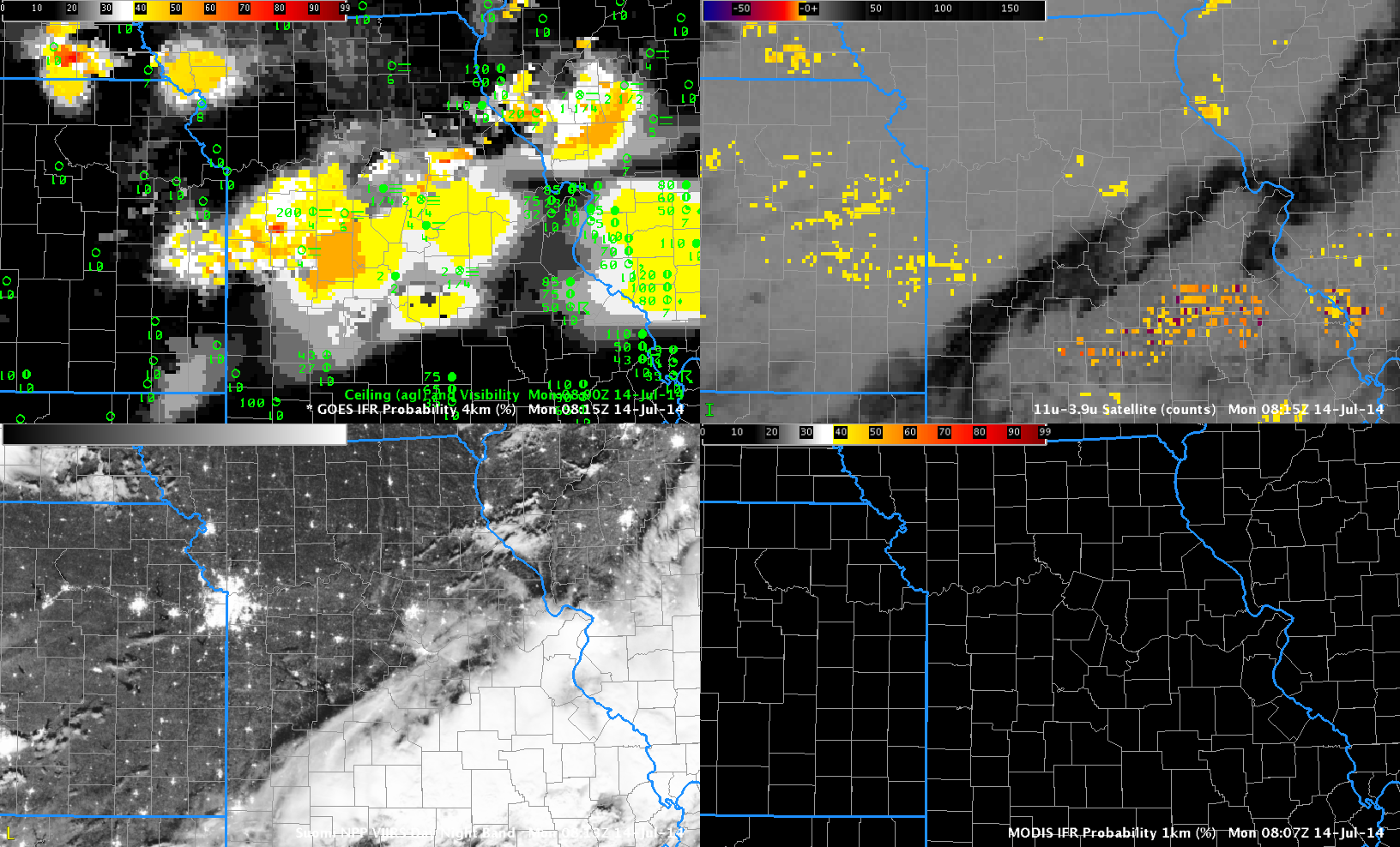
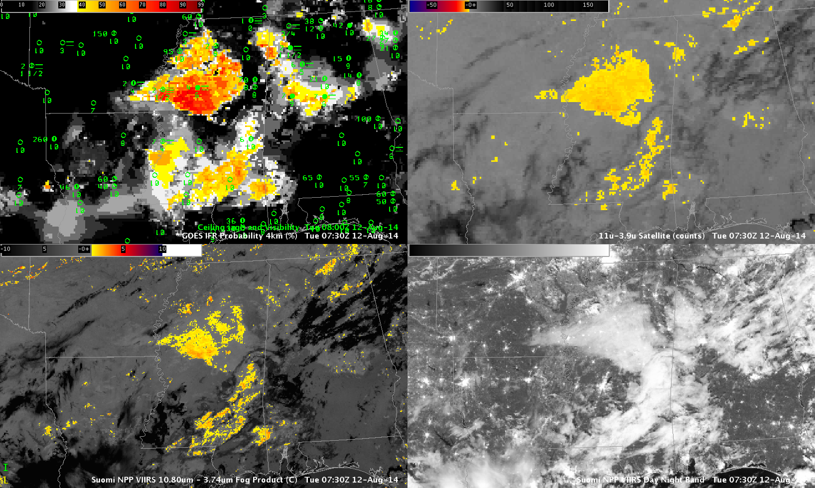
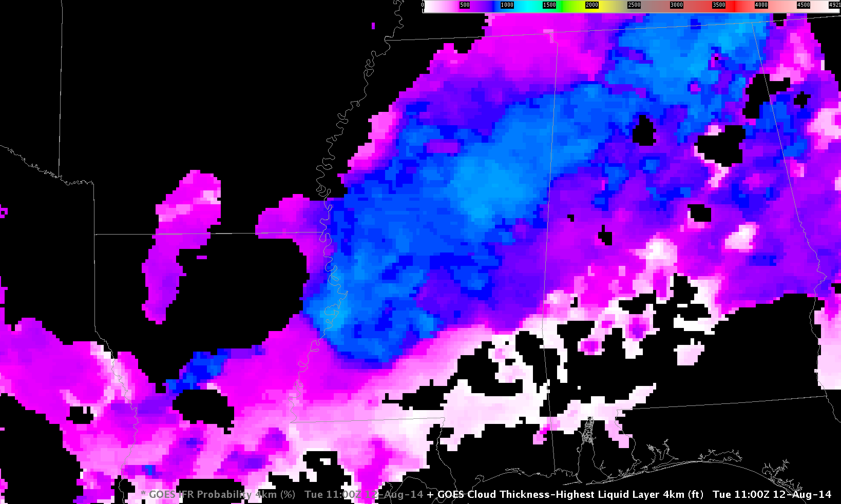
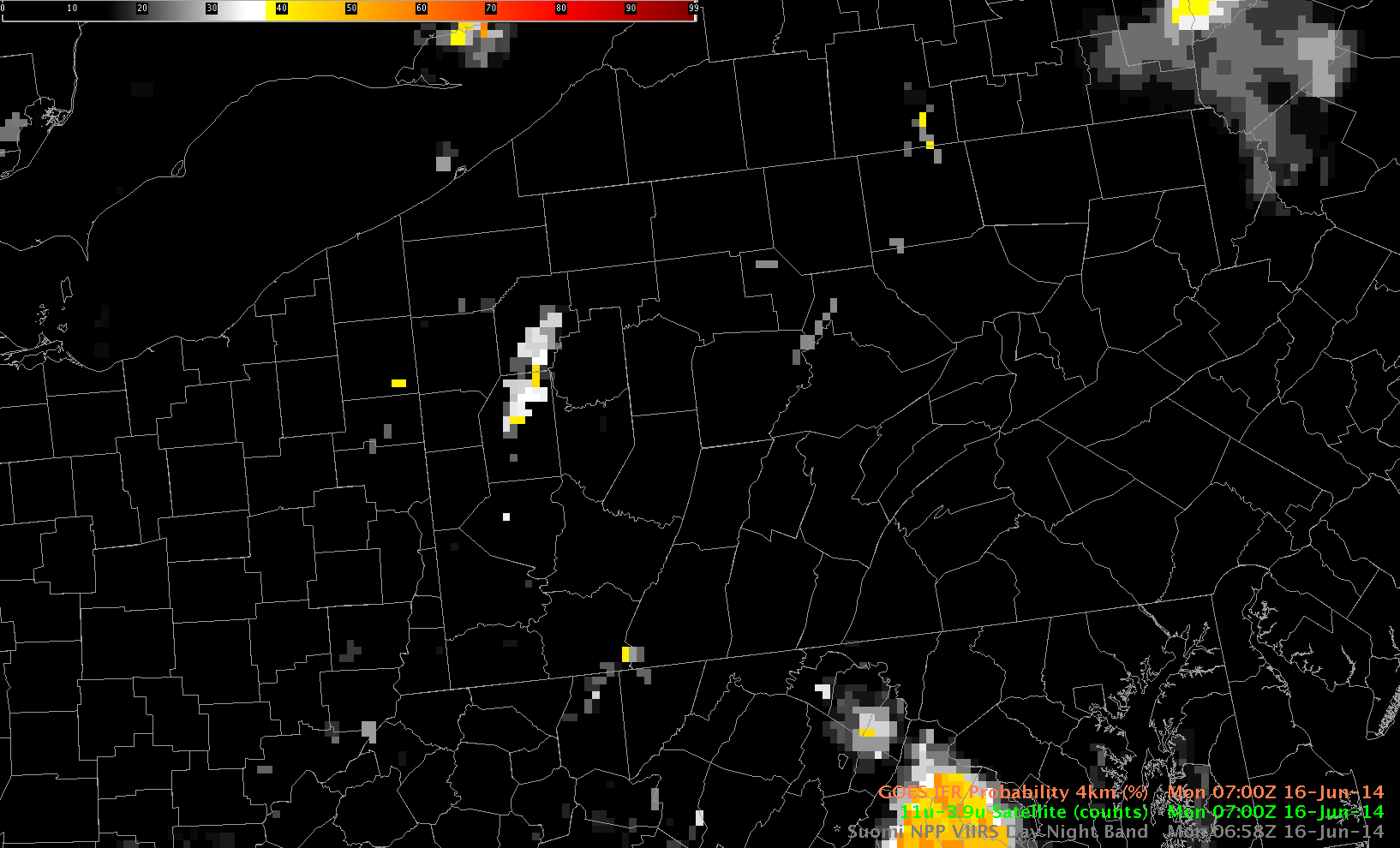
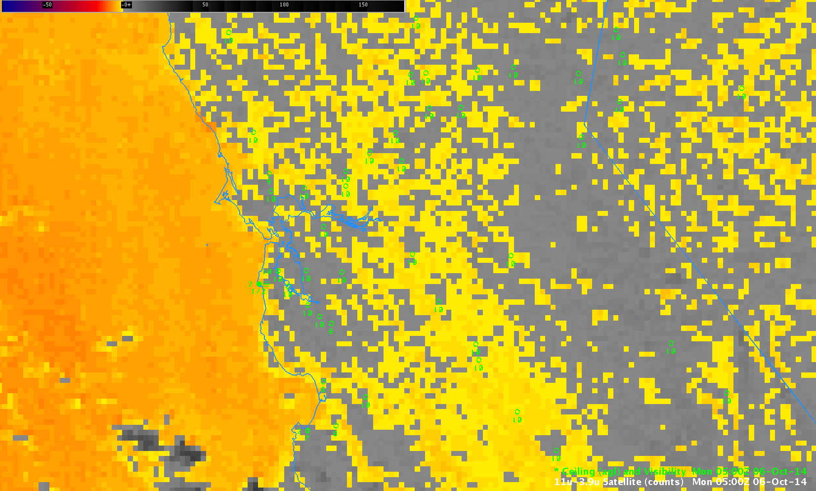
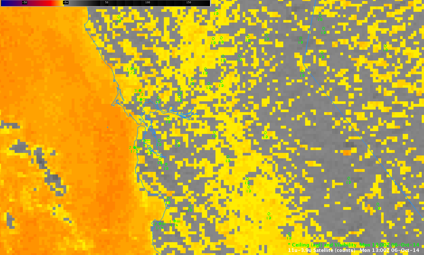
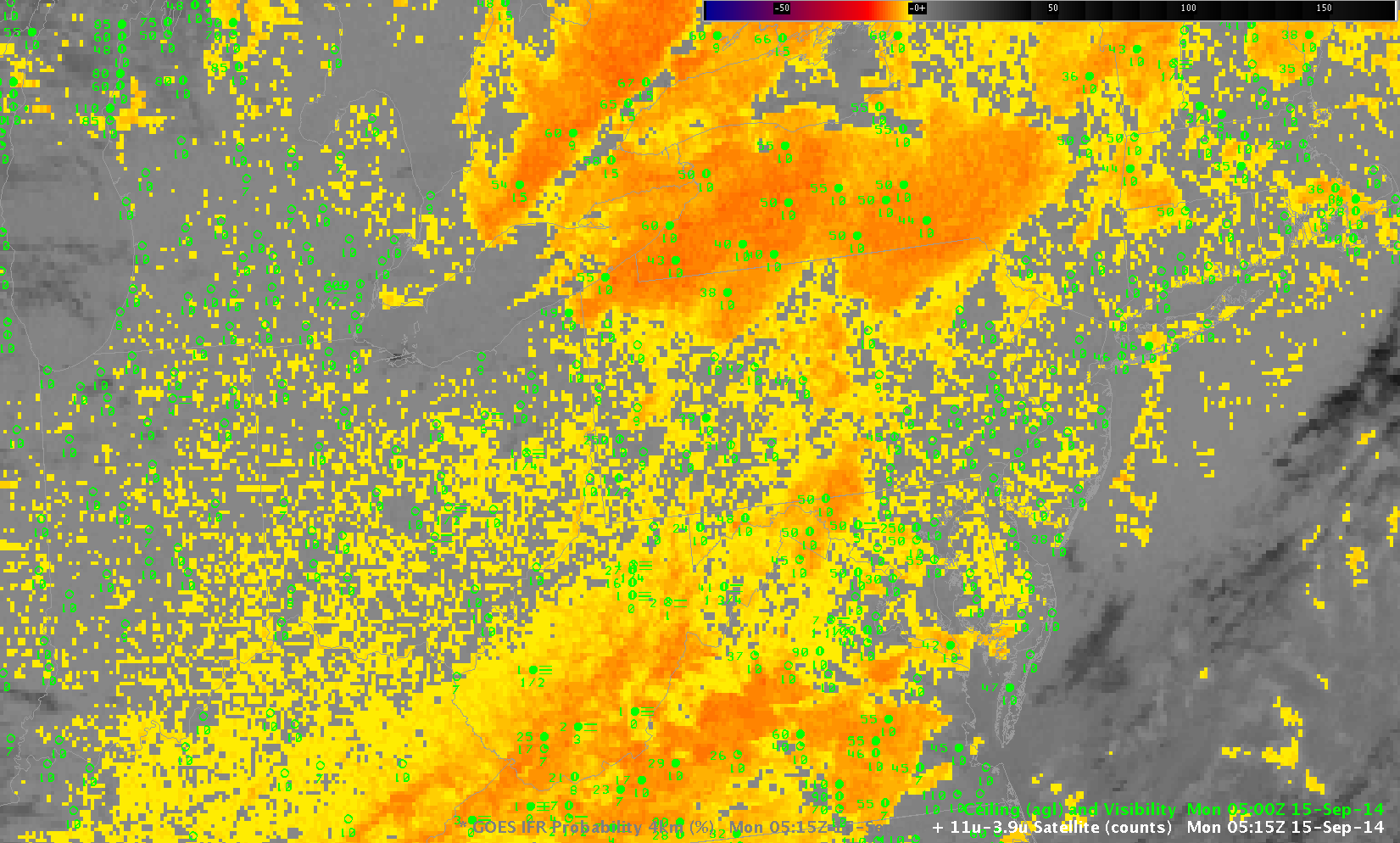
GOES-R IFR Probabilities (Upper Left), GOES-East Brightness Temperature Difference (10.7 µm – 3.9 µm) (Upper Right), Suomi/NPP Day/Night Band imagery (Lower Right), MODIS-based IFR Probabilitiy (Lower Left), times as indicated (Click to animate)

Moisture from departing late-day thunderstorms allowed for the development of dense fog over central Missouri overnight. The GOES-based IFR Probabilities, above, capture the low ceilings and reduced visibilities that developed. The traditional method of fog detection, the brightness temperature difference (BTD) between the 10.7 µm and 3.9 µm fields, was hampered by mid- and high-level clouds associated with the departing convection.

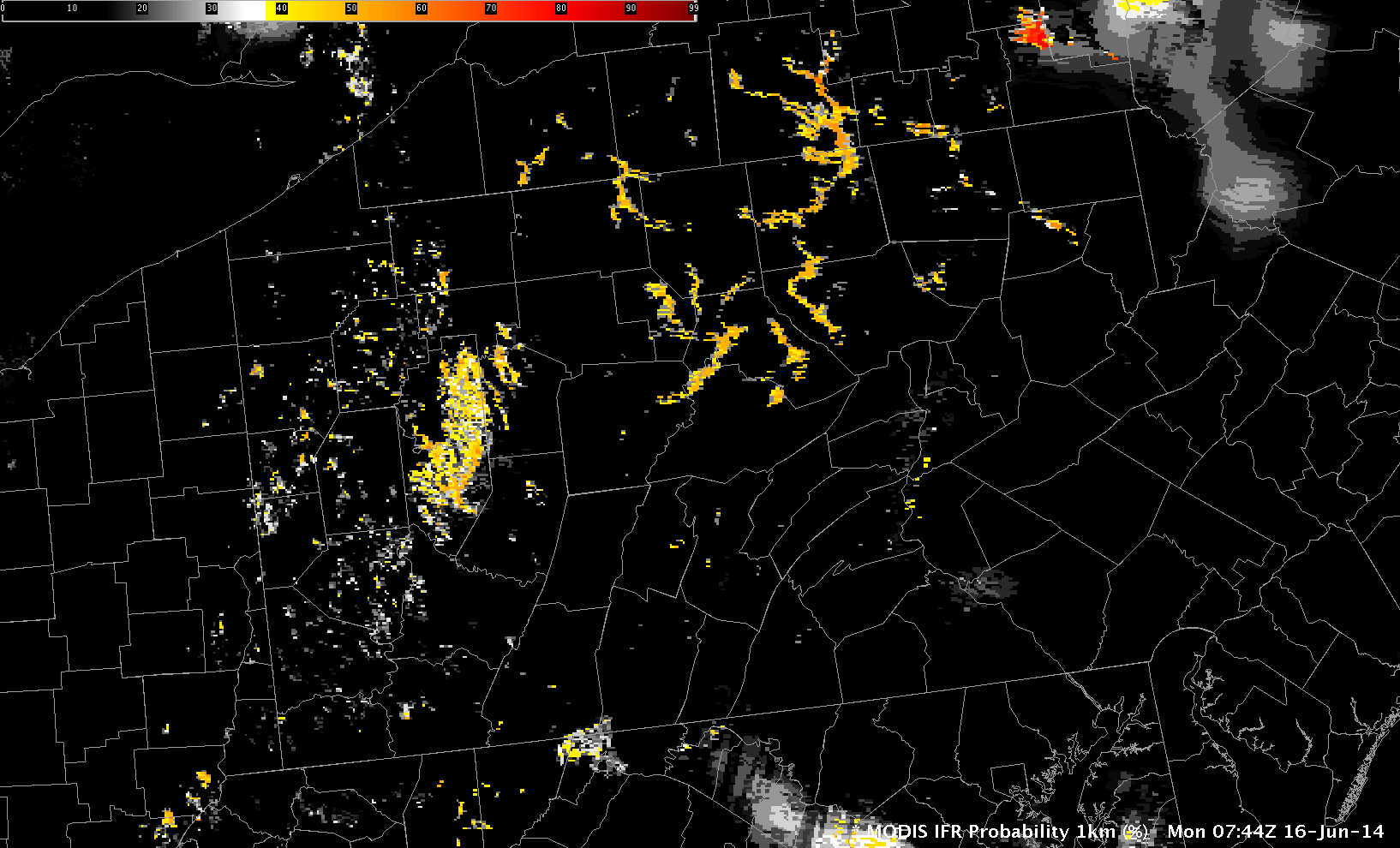
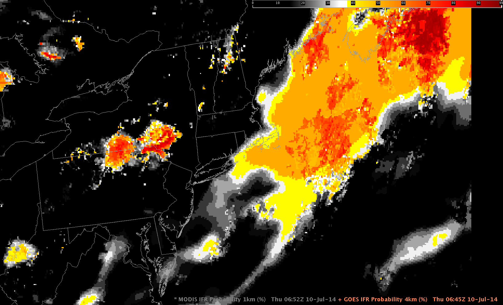
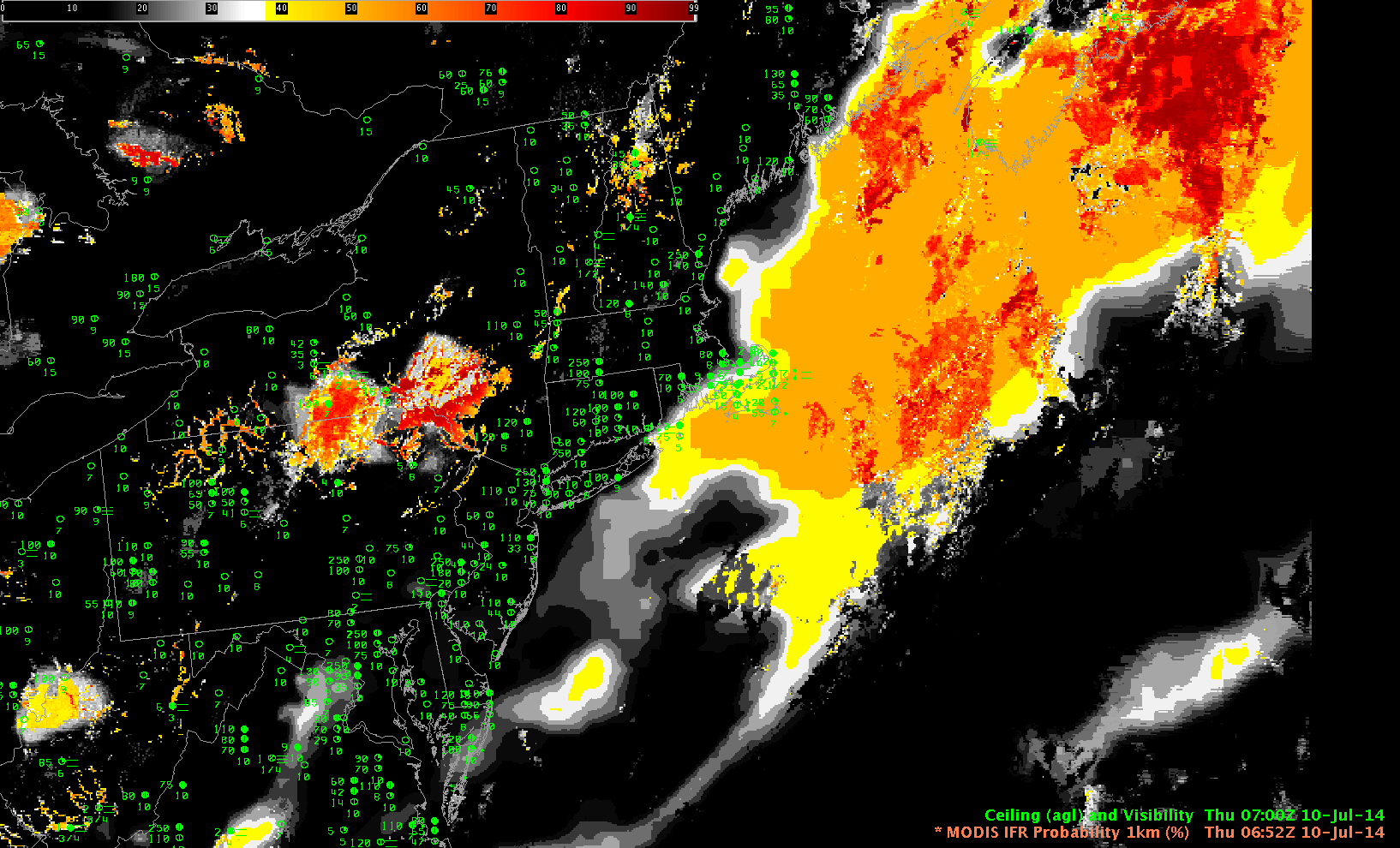
Polar-orbiting satellites such as Terra, Aqua and Suomi NPP can give high-resolution views of developing fog. In the present case, Terra overflew the region near 0400 UTC. The image below shows enhanced MODIS-based IFR Probabilities confined to central Missouri. An Aqua overpass at ~0800 UTC similarly gave a high spatial resolution view of the area. Of course, Terra and Aqua and Suomi NPP only give occasionaly snapshots. To see the ongoing development, temporal resolution as from GOES is key. But the polar orbiters can give an early alert if developing fog starts out at small scales that might be sub-pixel scale in GOES.

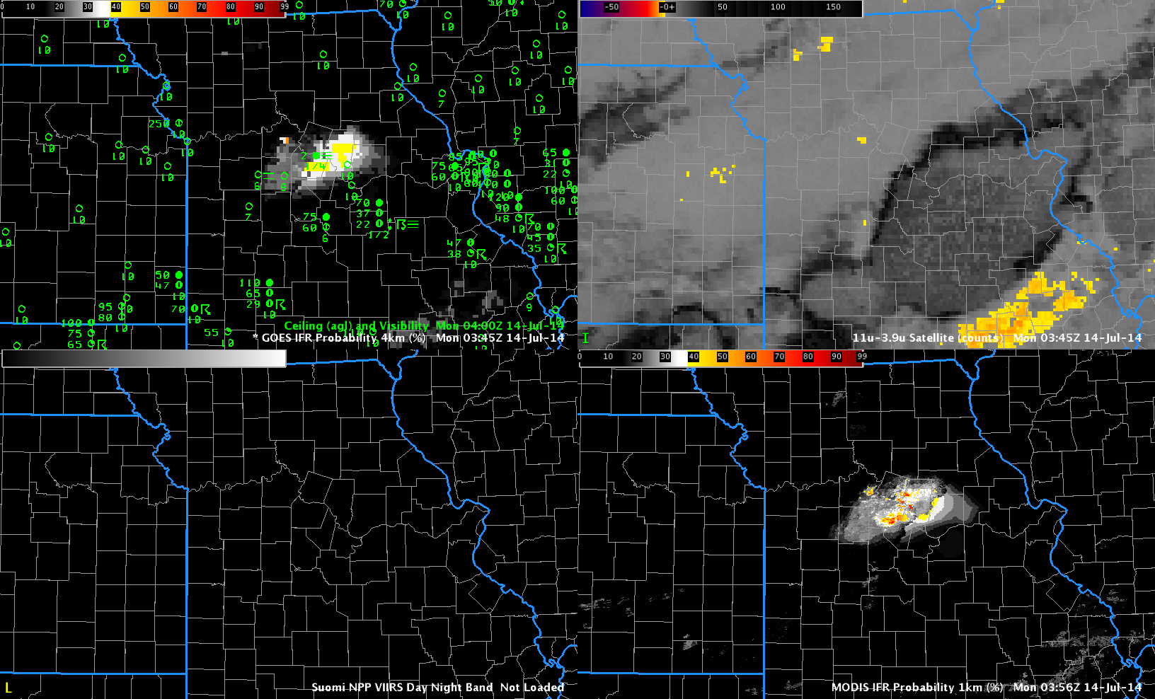
As above, but at 0400 UTC 14 July 2014 (Click to enlarge)

From the National Weather Service in St. Louis:

URGENT – WEATHER MESSAGE
NATIONAL WEATHER SERVICE ST LOUIS MO
527 AM CDT MON JUL 14 2014

MOZ041-047>051-059-141400-
/O.NEW.KLSX.FG.Y.0002.140714T1027Z-140714T1400Z/
BOONE MO-CALLAWAY MO-COLE MO-GASCONADE MO-MONITEAU MO-
MONTGOMERY MO-OSAGE MO-
INCLUDING THE CITIES OF…COLUMBIA…JEFFERSON CITY
527 AM CDT MON JUL 14 2014

…DENSE FOG ADVISORY IN EFFECT UNTIL 9 AM CDT THIS MORNING…

THE NATIONAL WEATHER SERVICE IN ST LOUIS HAS ISSUED A DENSE FOG
ADVISORY…WHICH IS IN EFFECT UNTIL 9 AM CDT THIS MORNING.

* TIMING…DENSE FOG HAS DEVELOPED AND WILL CONTINUE THROUGH 900
AM.

* VISIBILITIES…ONE QUARTER MILE OR LESS AT TIMES.

* IMPACTS…SIGNIFICANTLY REDUCED VISIBILITIES WILL LEAD TO
HAZARDOUS DRIVING CONDITIONS.

PRECAUTIONARY/PREPAREDNESS ACTIONS…

A DENSE FOG ADVISORY IS ISSUED WHEN DENSE FOG WILL SUBSTANTIALLY
REDUCE VISIBILITIES…TO ONE-QUARTER MILE OR LESS…RESULTING IN
HAZARDOUS DRIVING CONDITIONS IN SOME AREAS. MOTORISTS ARE ADVISED
TO USE CAUTION AND SLOW DOWN…AS OBJECTS ON AND NEAR ROADWAYS
WILL BE SEEN ONLY AT CLOSE RANGE.

The aviation portion of the AFD from St. Louis mentioned the probability of fog at 0800 UTC; the 1129 UTC update discussed the fog that was present over central Missouri:

.AVIATION: (For the 12z TAFs through 12z Tuesday Morning)
Issued at 609 AM CDT Mon Jul 14 2014

The first concern for this TAF package is that for low ceilings
and fog that have developed in the wake of precipitation that
exited the area overnight. In central MO and including KCOU, fairly
widespread dense fog has reduced visibilities to under 1/4SM for
much of the night. Further east and including metro area TAF sites,
trends indicate the potential for IFR cigs and MVFR visibility for
the first couple hours of the period. However, all sites affected
by fog should see an improvement through the morning hours as
ceilings lift and fog burns off. The second concern is that of a
second cold front, poised to move through the area today.
Currently, the cold front extends from roughly KDBQ southwestward
along the Missouri/Illinois border and just south of KAFK. While
showers may develop along the front as it moves through KUIN
during the late morning/early afternoon, greater instability
exists further south and east. Have currently continued VCSH
mention at KUIN and KCOU, and VCTS for metro TAF sites this
afternoon as the cold front moves through. Uncertainties regarding
coverage and exact timing preclude any TEMPO groups at this time.
The front should be south of all area TAF sites by 21Z, at which
time winds will have veered to the northwest and increased to
around 10-14KT. Winds will remain northwesterly through the end of
the period in the wake of the front, and while a mostly VFR
forecast is expected, reductions in ceilings/visibility may occur
with any storms that move over the terminals.

Distinguishing between stratus and fog over Pennsylvania

Suomi NPP 11.35 µm Infrared Imagery at 0609 and 0752 UTC, 10 July 2014 (Click to enlarge)

The orbital geometry of Suomi NPP allowed two high-resolution images of Pennsyvlania early in the morning of the 10th of July 2014. Can you tell from the imagery above if there is fog/stratus in the river valleys of Pennsyvlania? Are the relatively cool clouds from Pittsburgh northeastward towards Elmira, NY obstructing visibilities? Based on the IR (11.35 µm for Suomi NPP) imagery alone, above, that is a difficult question to answer. Historically, the brightness temperature difference between the longwave IR (11.35 µm) and the shortwave IR (3.74 µm) has been used to indentify water-based clouds. Imagery from Suomi NPP, below, highlights where water-based clouds (like stratus) exist. If the clouds are the same temperature as the surrounding land (likely the case for river fog), a single 11.35-µm image is of little help in identifying the clouds.

Suomi NPP 11.35 – 3.74 µm Brightness Temperature Difference at 0609 and 0752 UTC, 10 July 2014 (Click to enlarge)

The Day-Night band can also highlight where clouds exist, because lunar illumination reflects well off clouds. A 3/4-full moon ably illuminates the scene at 0609 UTC, but that moon has set at 0747 UTC and the Clouds are harder to see.

Suomi NPP Day/Night Band at 0609 and 0752 UTC, 10 July 2014 (Click to enlarge)

Both the Day/Night band and the Brightness Temperature Difference Fields (and any Infrared image) gives information about the top of the cloud. Fog existence is difficult to discern only from satellite data because the bottom of the cloud is not sampled. This is why a fused product (such as IFR Probability) that includes surface information (in the case of IFR Probability from the Rapid Refresh Model) is desirable. MODIS data can be used to compute IFR Probability, and a MODIS-carrying Aqua pass occurred in between the two Suomi NPP Passes shown above.

MODIS 11 – 3.9 µm Brightness Temperature Difference and IFR Probability at 0652 UTC, 10 July 2014 (Click to enlarge)

In the two images above, note how the IFR Probability Fields de-emphasize the low cloud areas that stretch northeastward from Pittsburgh towards Elmira. This is likely mid-level stratus. River Fog over northeast Pennsylvania is highlighted in the IFR Probability fields (and in the brightness temperature difference field). This image, which shows the GOES-based IFR Probability field at 0645 UTC, highlights the power of MODIS’ superior spatial resolution in the early detection of small-scale fog. The large region of reduced visibility around Elmira NY (meager surface observations suggest this large region of fog verified) appears in both MODIS- and GOES-based IFR Probability fields. Only the MODIS-based IFR Probability field, however, has a distinct river-valley signal over northeast Pennsylvania.

MODIS and GOES IFR Probability both suggest IFR conditions may be occurring over the Atlantic Ocean. The brightness temperature difference field shows no low cloud signal there because of a cirrus shield. IFR Probability gives a signal of fog here based on information from the Rapid Refresh.

Fog in the Valleys of Pennsylvania and New York

Suomi/NPP Day/Night Band and Brightness Temperature Difference (11.35 – 3.74) at 0658 UTC on 16 June 2014 (Click to enlarge)

Suomi/NPP Day/Night band “Visible Imagery at Night” from last night at 3 AM EDT over Pennsylvania and surrounding states shows cloud formation in the river valleys of Pennsylvania and New York. The brightness temperature difference also shows these cloud formations, but note over eastern New York how high cirrus prevents the detection of low clouds in river valleys using the brightness temperature difference field, but the cirrus is thin enough that the Day/Night band does show the low clouds. The brightness temperature difference field can show where clouds are present in regions where city lights in the day/night band might appear similar to clouds on a night when lunar illumination is strong (as was the case on 16 June 2014) — for example, along US Highway 220 from Lock Haven to Jersey Shore and Williamsport in southern Clinton and Lycoming Counties.

Of course, the Suomi/NPP satellite is seeing the top of the cloud, so it can be difficult to infer ceiling and visibility obstructions from these data. The GOES-based IFR Probability field from about the same time, below, shows hints of visibility restrictions, but the coarser resolution of GOES-13 (compared to Suomi/NPP) limits the ability of GOES to herald the development of fog. In addition, the 13-km resolution of the Rapid Refresh model data that are also used in the GOES-R IFR Probability fields is insufficient to resolve the small river valleys (such as Pine Creek that shows up very well in the S/NPP imagery in western Lycoming County). Portions of the Susquehanna River basins do show marginally enhanced probabilities, certainly something that would alert a forecaster to the possibilities of fog.

GOES-based IFR Probabilities, 0700 UTC on 16 June 2014 (Click to enlarge)

MODIS data can also be used to produce IFR Probabilities at infrequent intervals, but a timely overpass at 0744 UTC shows high probabilities in most of the river valleys of central Pennsylvania and upstate New York, with the highest probabilities near Elmira, NY.

MODIS-based IFR Probabilities, 0744 UTC on 16 June 2014 (Click to enlarge)

The GOES-R IFR Probabilities at 1000 UTC, below, show evidence that the fog/low stratus have become widespread enough in river valleys to be detected even by GOES. Elmira, NY, is reporting IFR conditions, and such conditions are also likely elsewhere in the valleys (although no observations are available to confirm that).

GOES-based IFR Probabilities, 1000 UTC on 16 June 2014 (Click to enlarge)

Use timely polar-orbiting satellite data — with high resolution — to confirm suspicions of developing fog in river valleys. Then monitor the situation with the good temporal resolution of GOES. During the GOES-R era, geostationary satellite spatial resolution will be increased and fog detection from GOES-R should occur with better lead time.

Terrain and IFR Probabilities

GOES-R IFR Probabilities computed from GOES-West at 0930 UTC on 28 May, and Color-enhanced terrain (Click image to enlarge)

When IFR Probabilities are enhanced over high terrain, how confident can you be that IFR conditions are occurring? Surface observations are rare on mountain tops. It’s possible that clouds occurring are at one level as the terrain rises up into the clouds, and ceilings at adjacent stations can give an indication of the cloud base (in the present case, ceilings are about 9000 feet above sea level at Seattle, for example).

Suomi/NPP Day/Night band imagery can verify that clouds exist in the region where IFR Probabilities are elevated. The toggle below, of Day/Night band and Brightness Temperature Differences, shows compelling evidence (even in low light conditions) of clouds along the spine of the mountains in central Washington and Oregon.

Suomi/NPP VIIRS Day/Night Band and Brightness Temperature Difference (11.45 µm – 3.74 µm), 0935 UTC on 28 May (Click to enlarge)

High-resolution MODIS data are also used to produce IFR Probabilities, and they can be used to deduce the presence of low ceilings/reduced visibilities as well. The toggle below, from 1027 UTC, shows the brightness temperature difference field (11.0 – 3.9) from MODIS and the IFR Probability field. It is likely in this case that high clouds were shrouding the higher peaks of the Cascade Mountains.

GOES-R Fog Product Examples

Fog detection fusing GOES, Terra/Aqua or Suomi/NPP Satellite data with Model output