 |
||
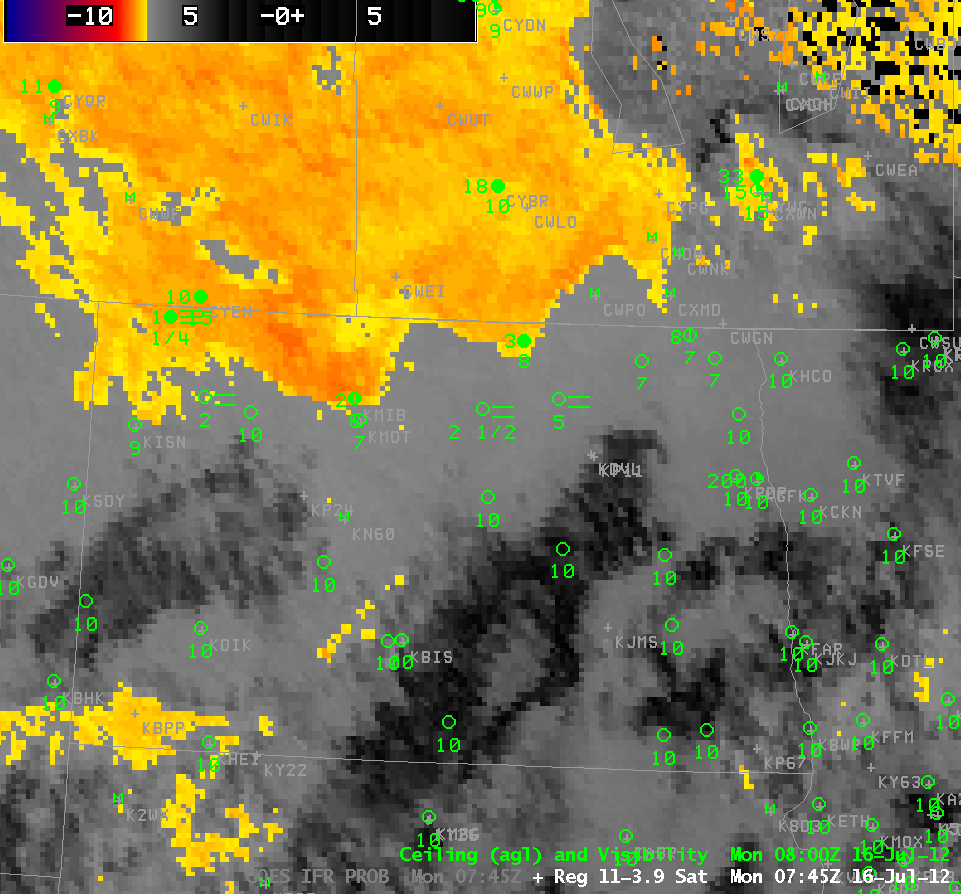
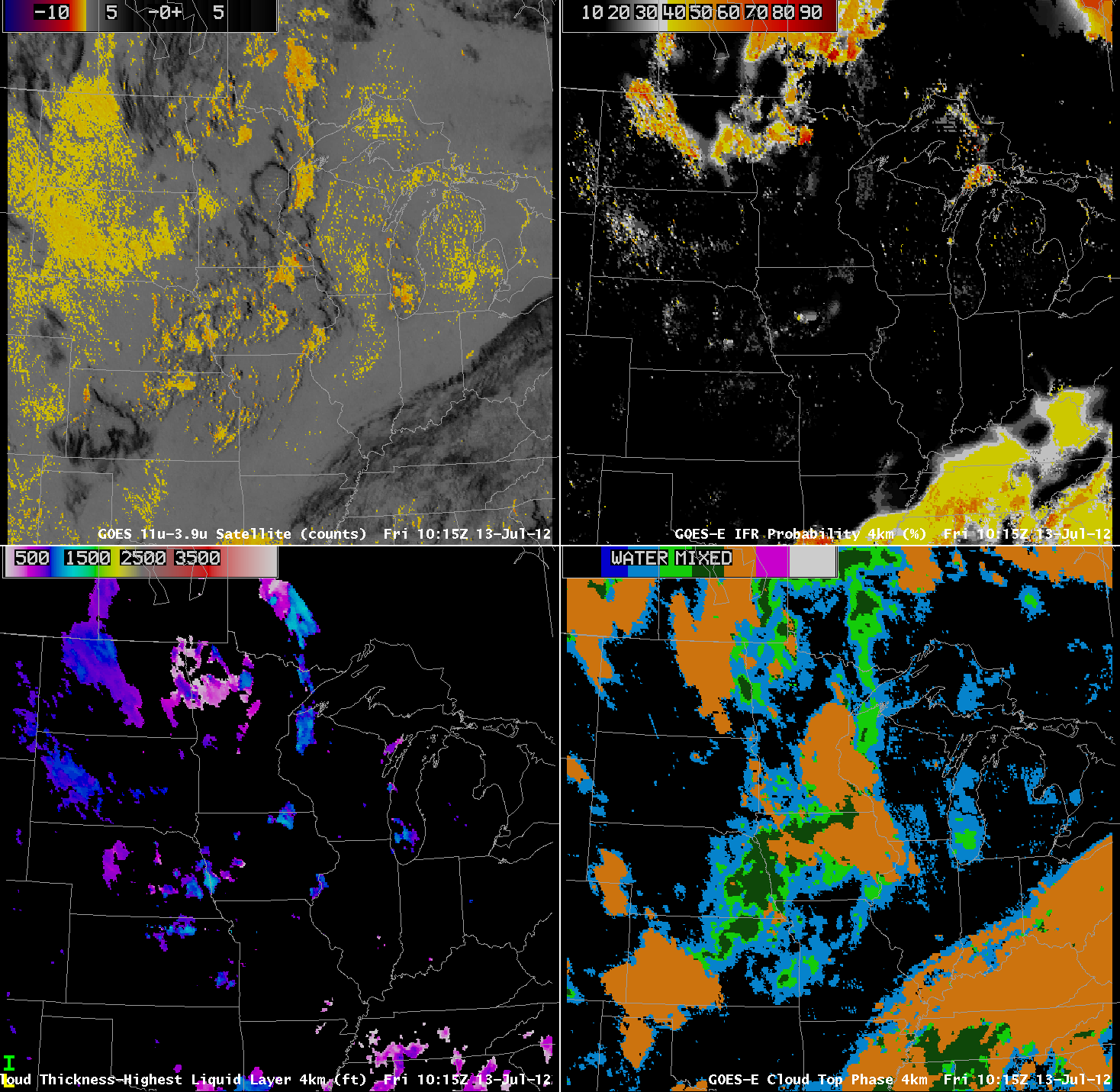
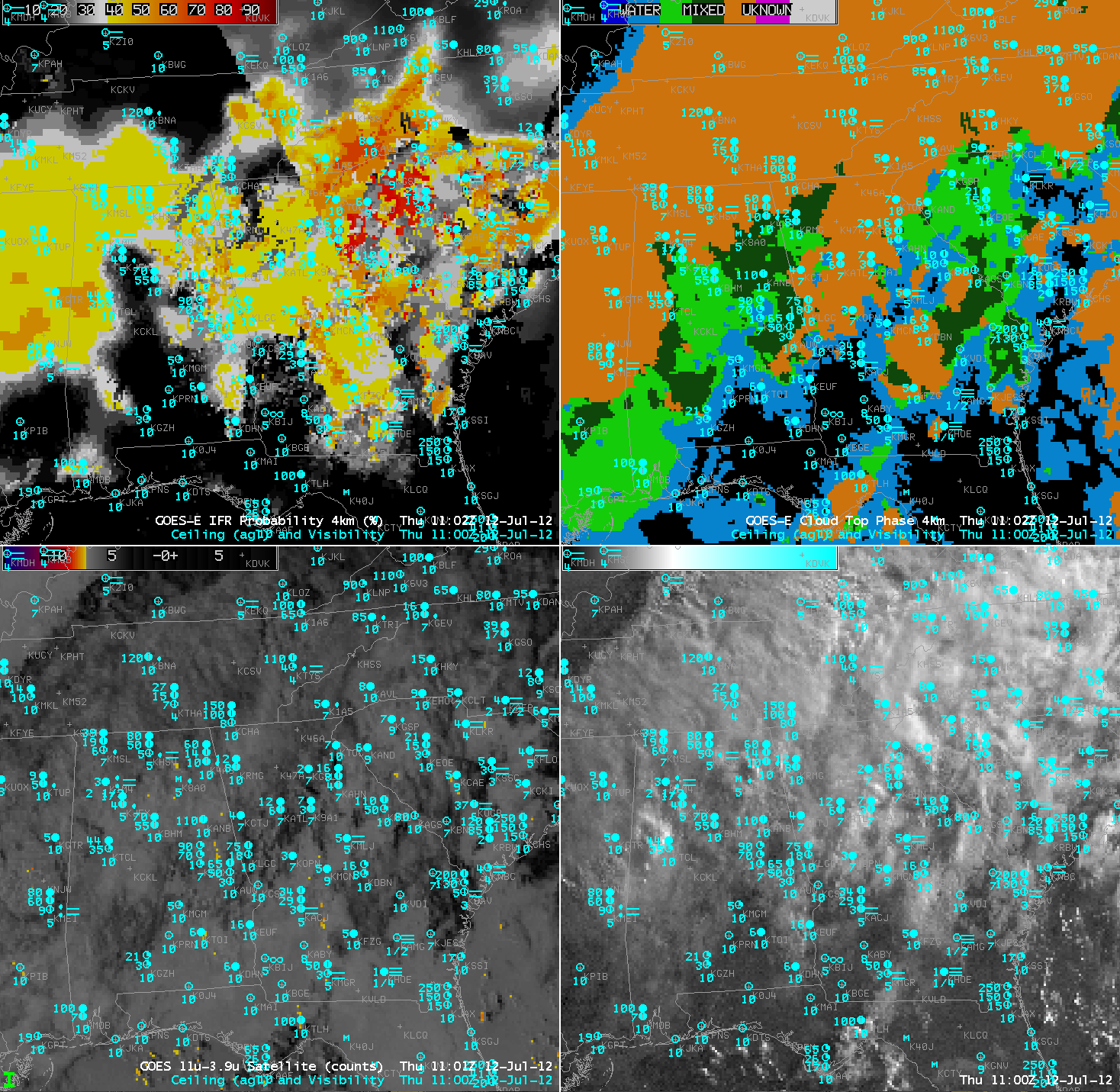
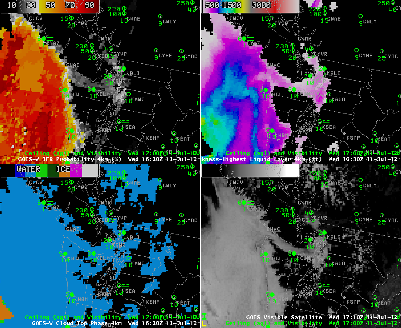
| GOES-R IFR Probabilities computed using MODIS data (upper left), MODIS Brightness Temperature Difference (the ‘traditional’ Fog Product) (upper right), Lowest 1km Relative Humidity from the NAM (lower left), MODIS IR Window Channel (lower right) |
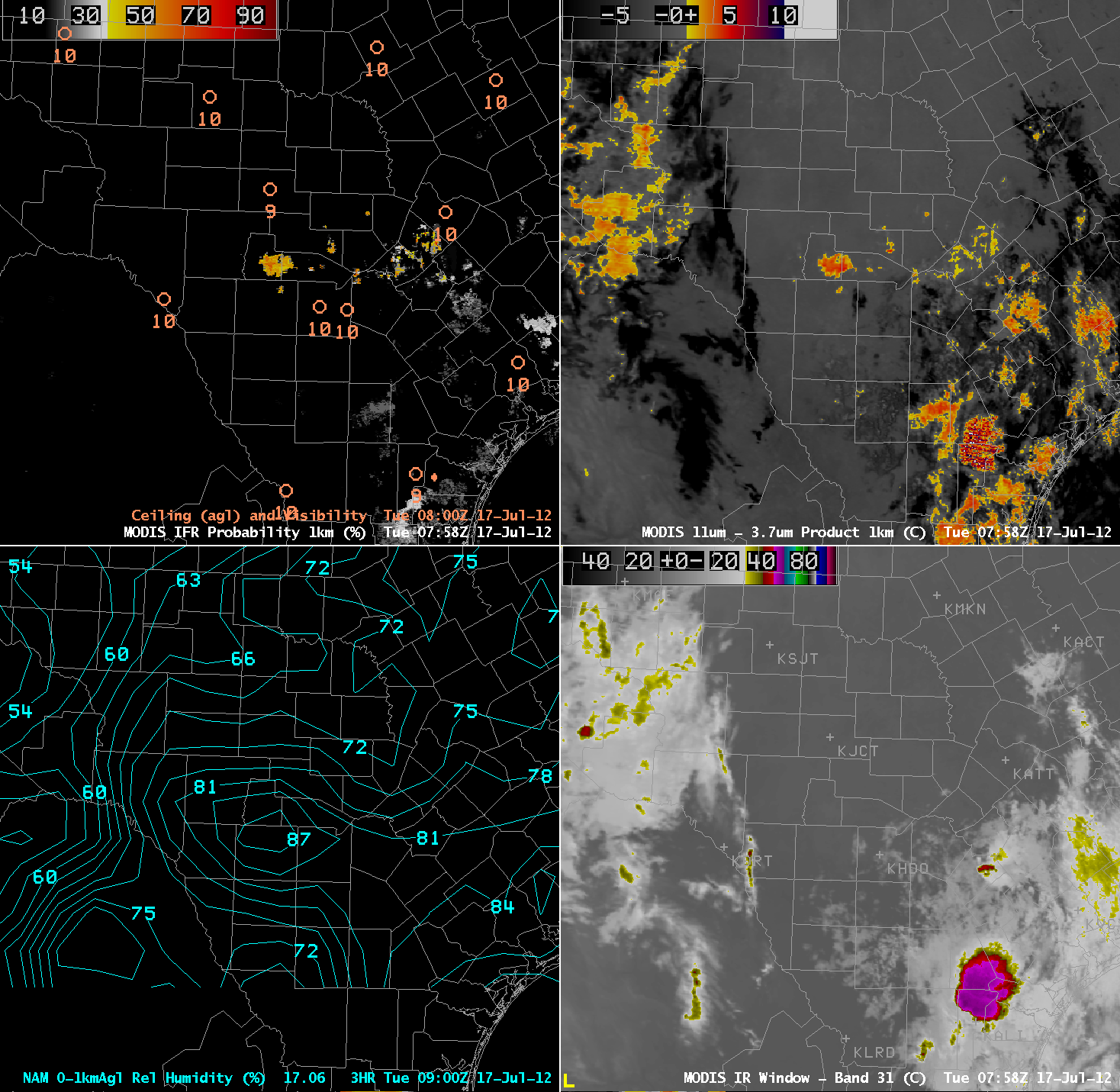
The MODIS-based GOES-R IFR probability image, above, showed a region of high probabilities of IFR over Bandera and Real Counties in Texas west of San Antonio. This signal is driven by the brightness temperature difference (shown, upper right) and the relative humidity in the Rapid Refresh. The NAM relative humidity is shown in the lower left image, and the signal in the GOES-R IFR field suggests the RAP relative humidity is similar. Note how the brightness temperature difference signal farther west in the image does not lead to a signal in the IFR Probabilities; model relative humidities there are lower.
Does the high probability of IFR signal verify? In other words, when you see an isolated signal like this, how much credence can you give it? Hondo, TX (HDO), just southeast of the higher IFR probabilities, does not show IFR conditions. How do things evolve with time? GOES-based imagery, below, show the expansion of the IFR probabilities from 0800 UTC, the approximate time of the MODIS pass, above, to 1030 UTC. The expansion is typical of what would occur with radiational fog formation overnight. By 1100 UTC, ceilings at Hondo (HDO) and Rocksprings (ECU) are near IFR conditions. It appears that the IFR probability signal is correctly diagnosing the slow development of a fog/stratus deck.
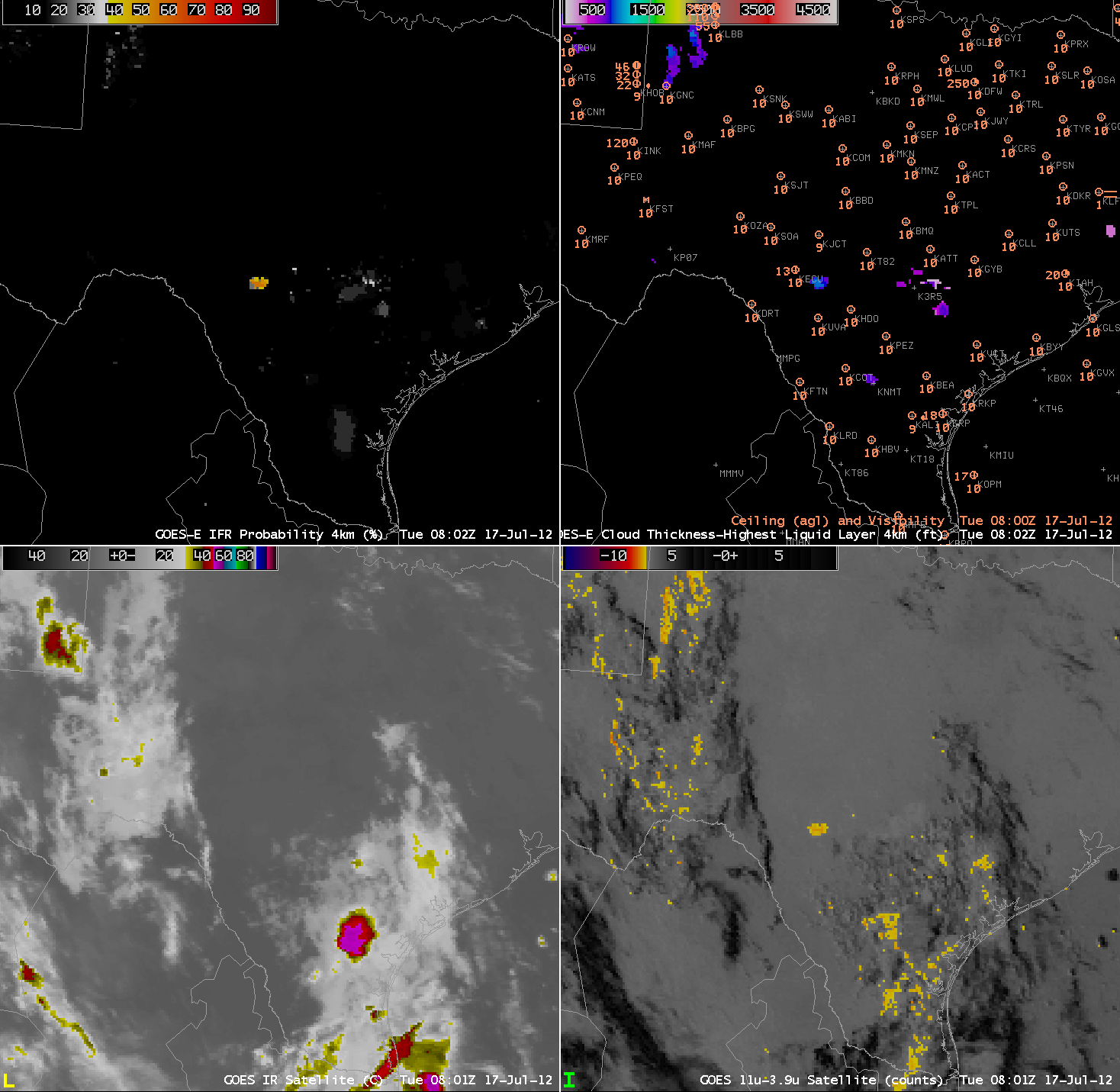 |
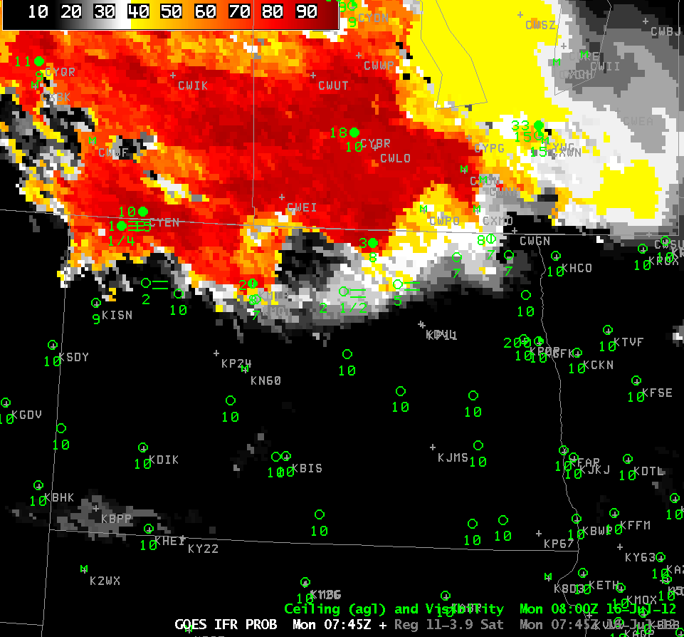
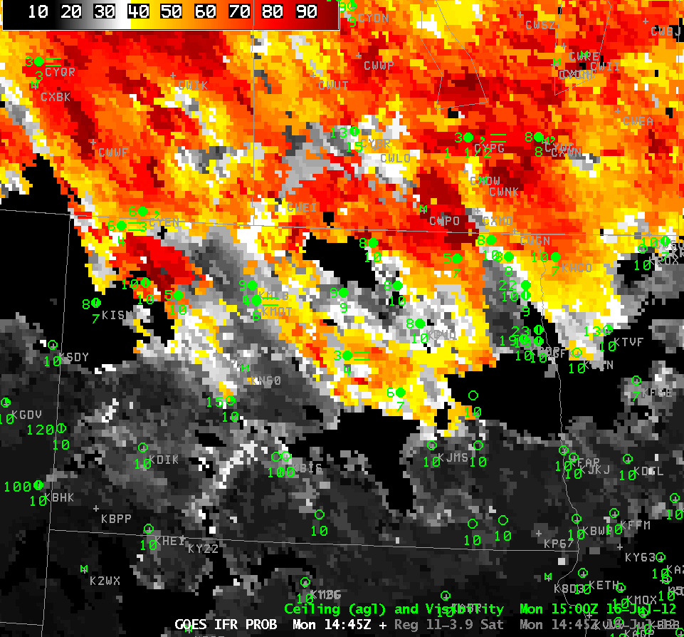
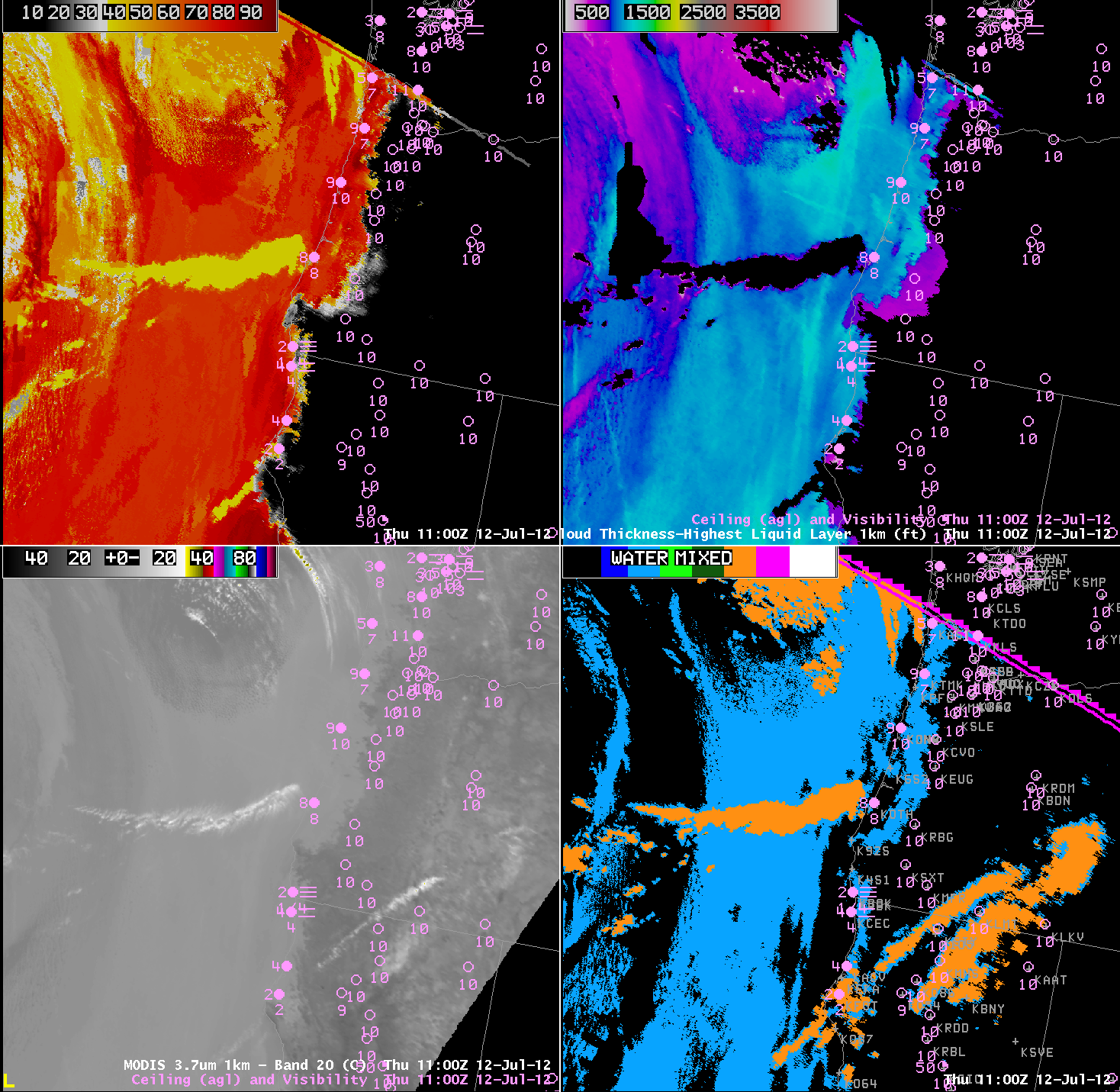
| GOES-R IFR Probabilities (Upper left), Ceilings and Visibility plotted over GOES-R Cloud Thickness (upper right), GOES-East enhanced Window Channel brightness temperature (bottom left), GOES-East Brightness Temperature Difference (bottom right) from 0800 UTC |
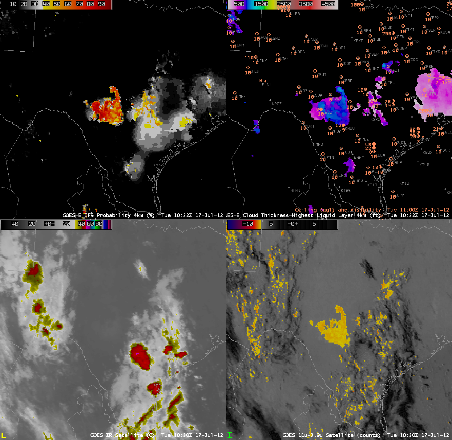 |
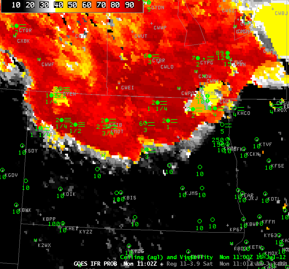
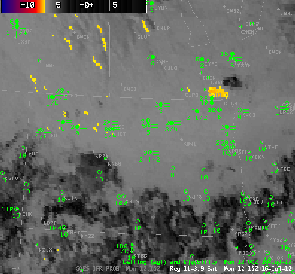
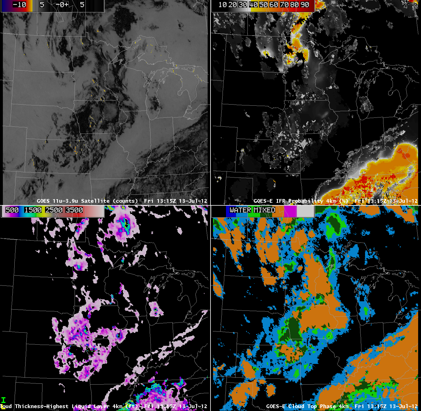
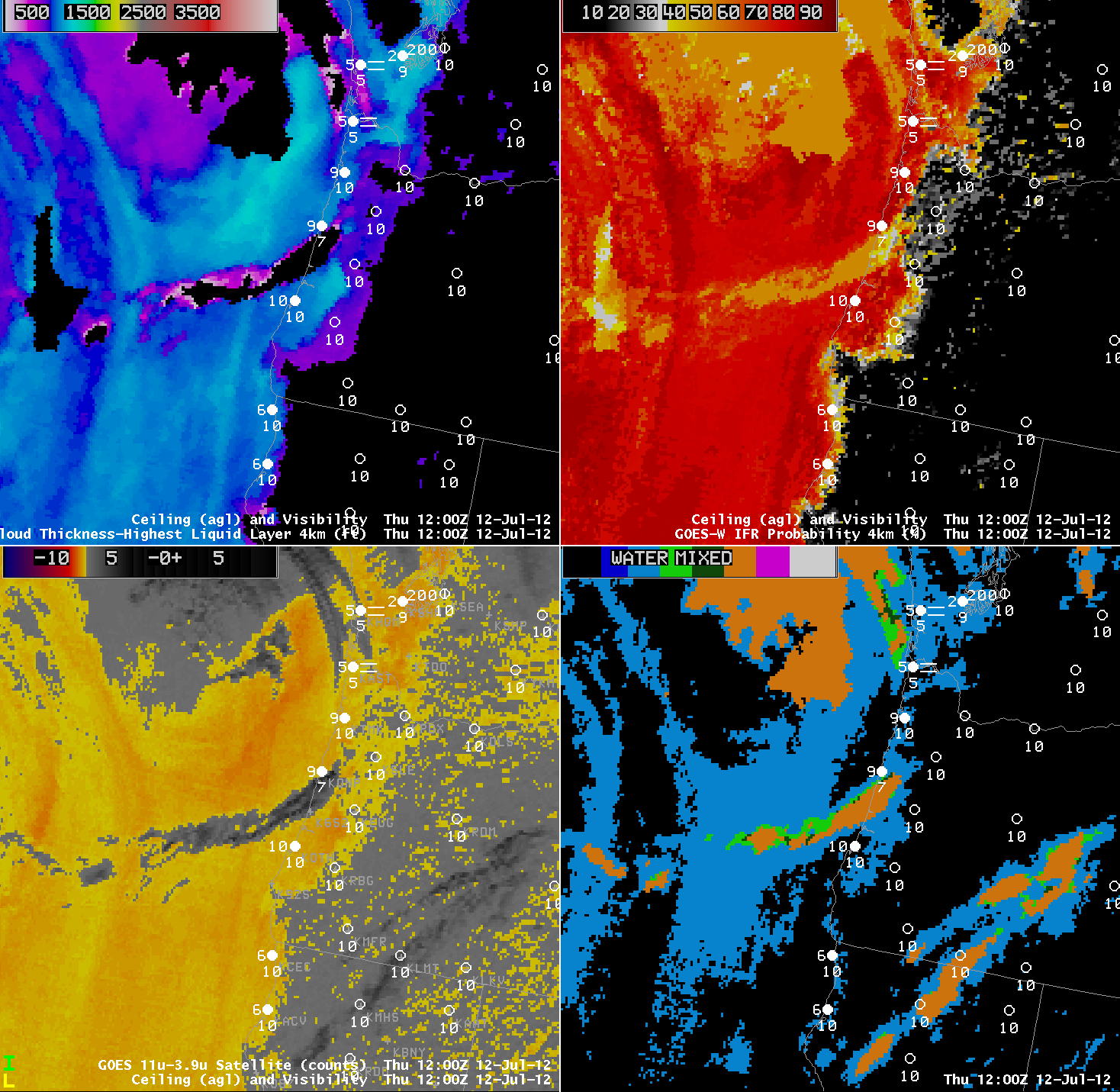
| GOES-R IFR Probabilities (Upper left), Ceilings and Visibility plotted over GOES-R Cloud Thickness (upper right), GOES-East enhanced Window Channel brightness temperature (bottom left), GOES-East Brightness Temperature Difference (bottom right) from 1030-1100 UTC |
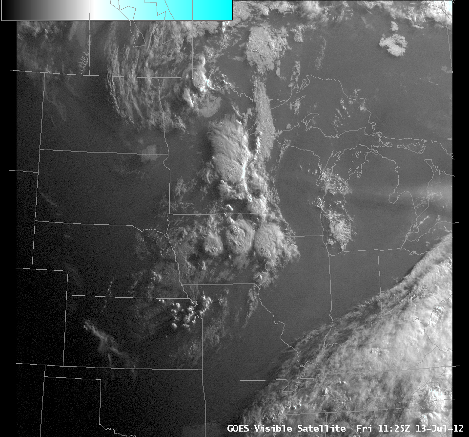
There was a fortuitous pass of the Suomi/NPP satellite over this region as the fog/low stratus developed. Does that satellite give any more information about the presence of fog? The loop below toggles between the GOES-R IFR probability from GOES-East data and the Day/Night Band from VIIRS. Because the Moon is nearly new, very little moonlight is illuminating the cloud field so it is difficult to determine if fog is actually present at 0832 UTC over the region. The parts of the counties over which the fog is developing are sparsely populated, so there are no city lights from which to glean information.