Category Archives: Multiple Cloud Layers

IFR Conditions with cold-season extratropical cyclones

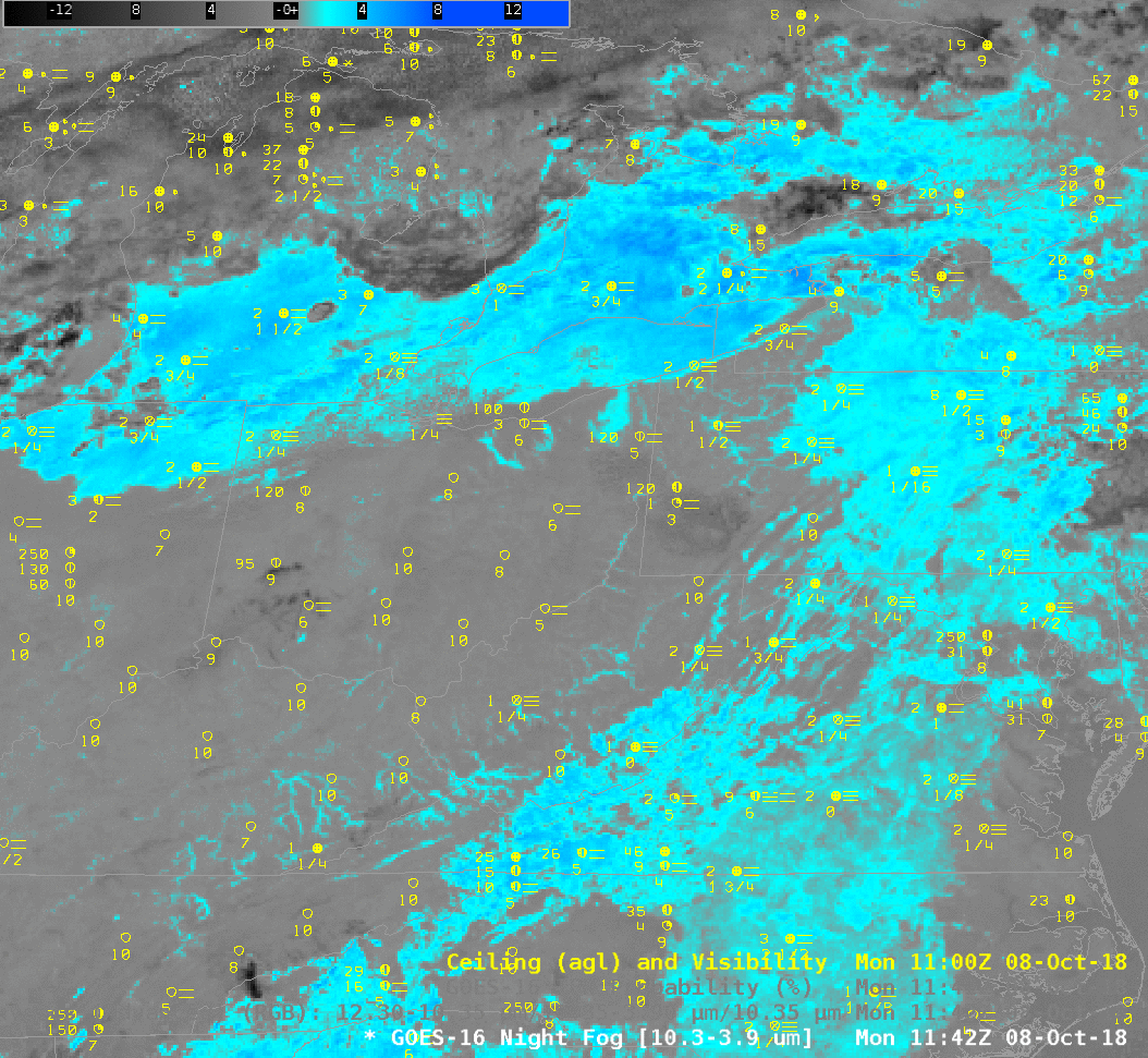
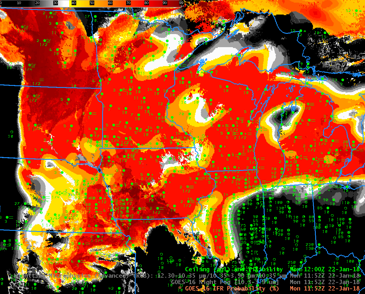
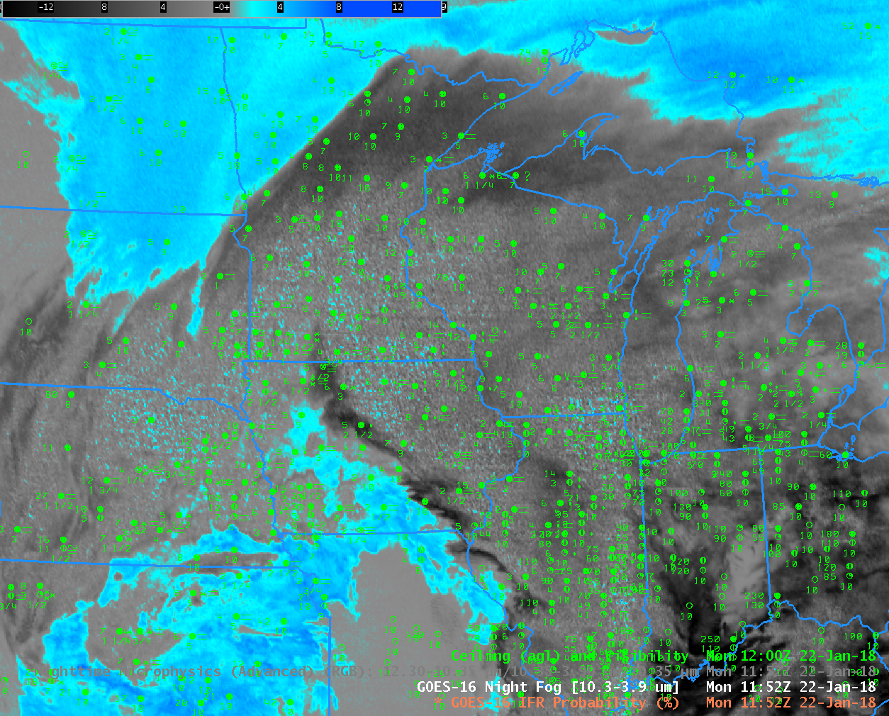
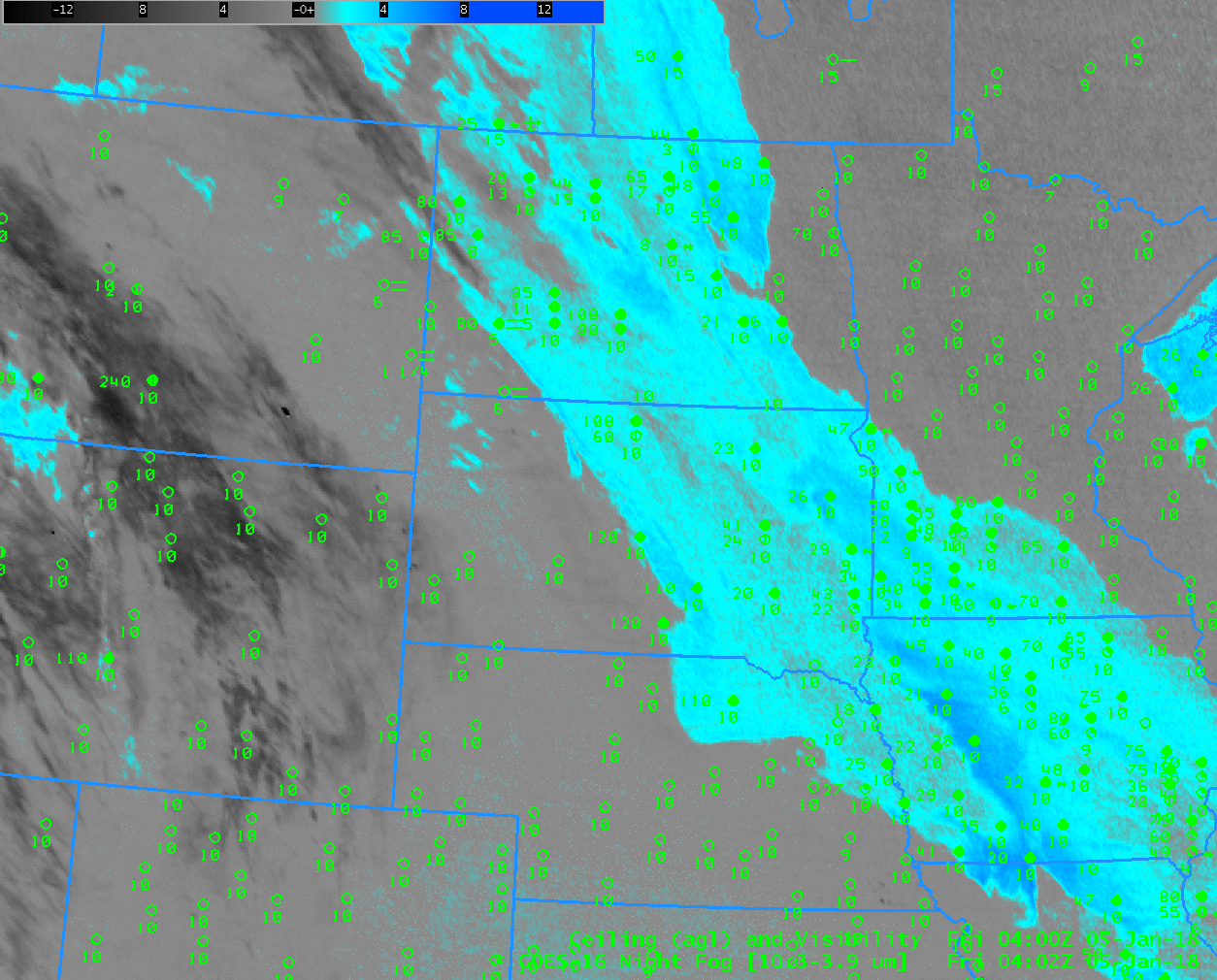
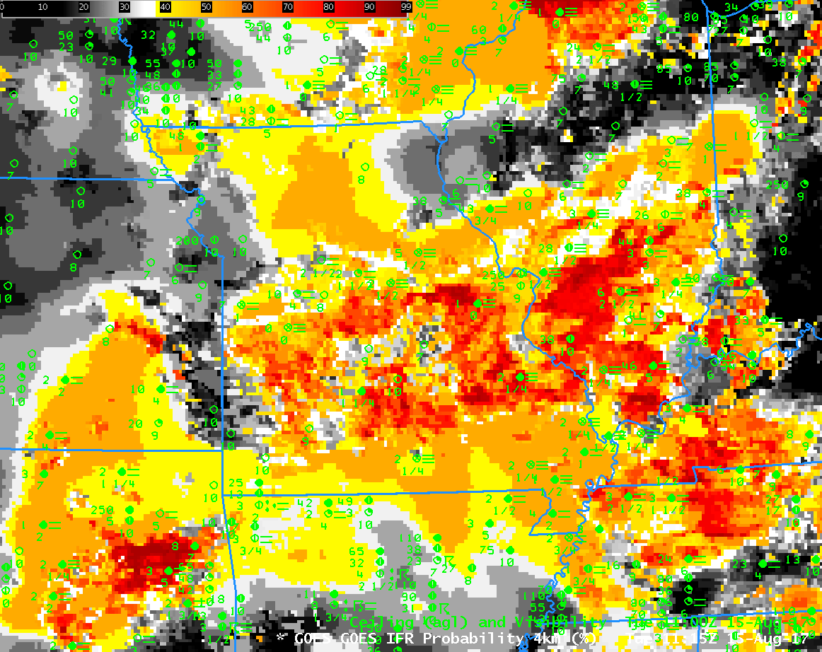
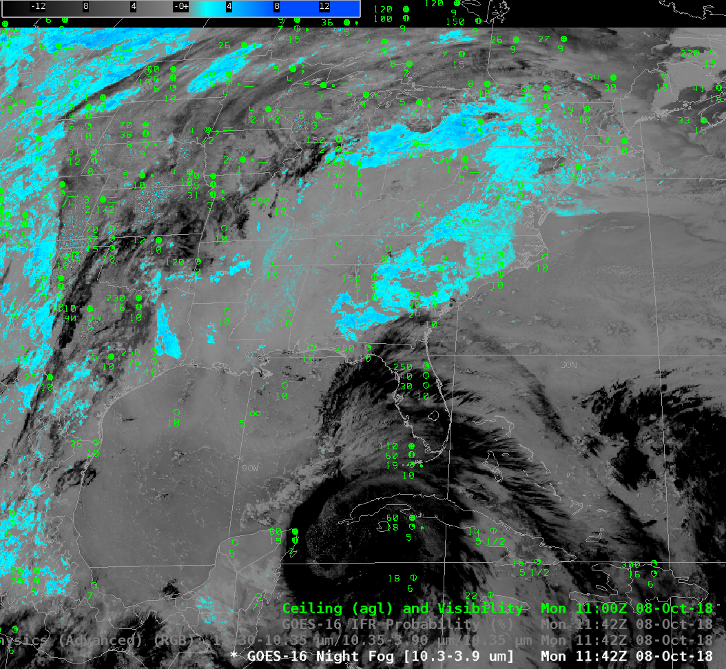
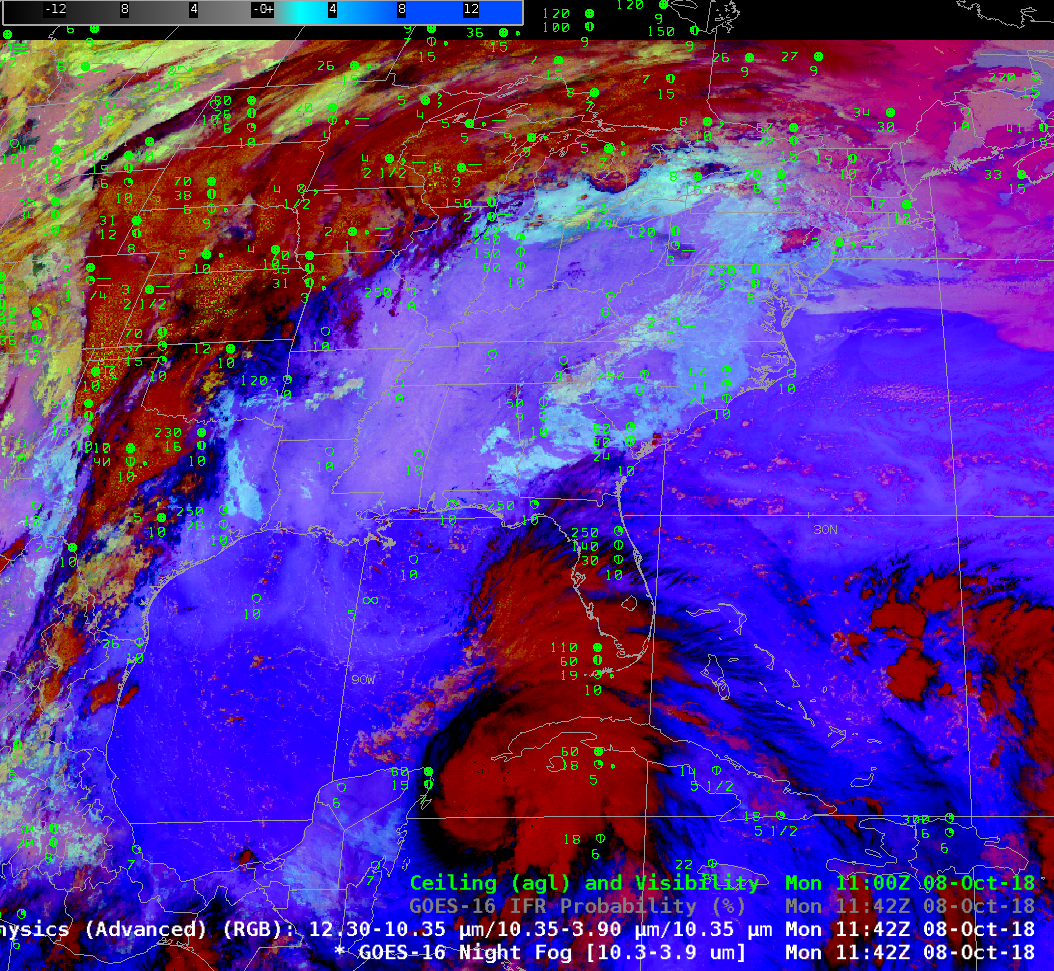
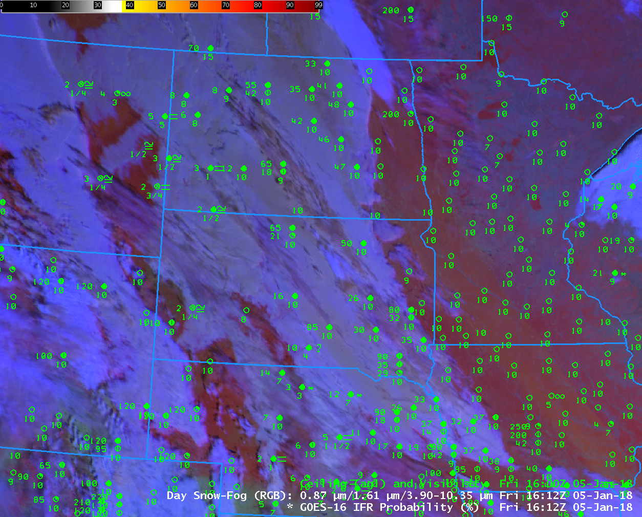
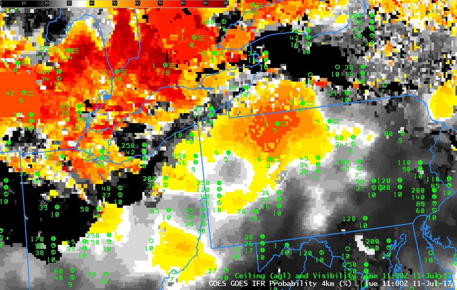
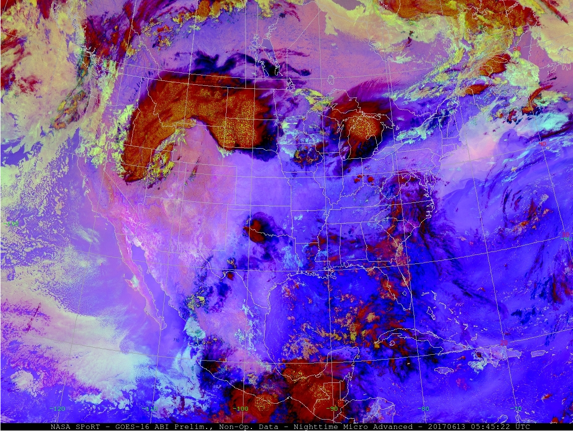
GOES-16 Night Fog Brightness Temperature Difference (10.3 µm – 3.9 µm), Advanced Night Time Microphysics RGB, and GOES-16 IFR Probability fieds at 1142 UTC on 8 October 2018 (Click to enlarge)

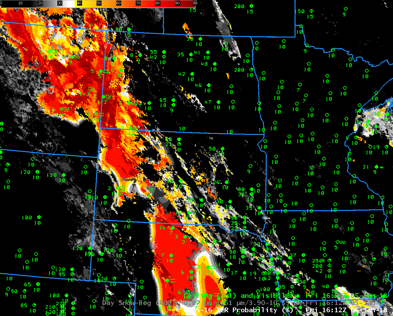
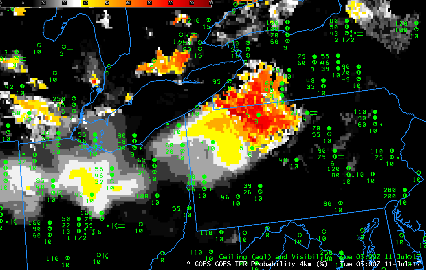
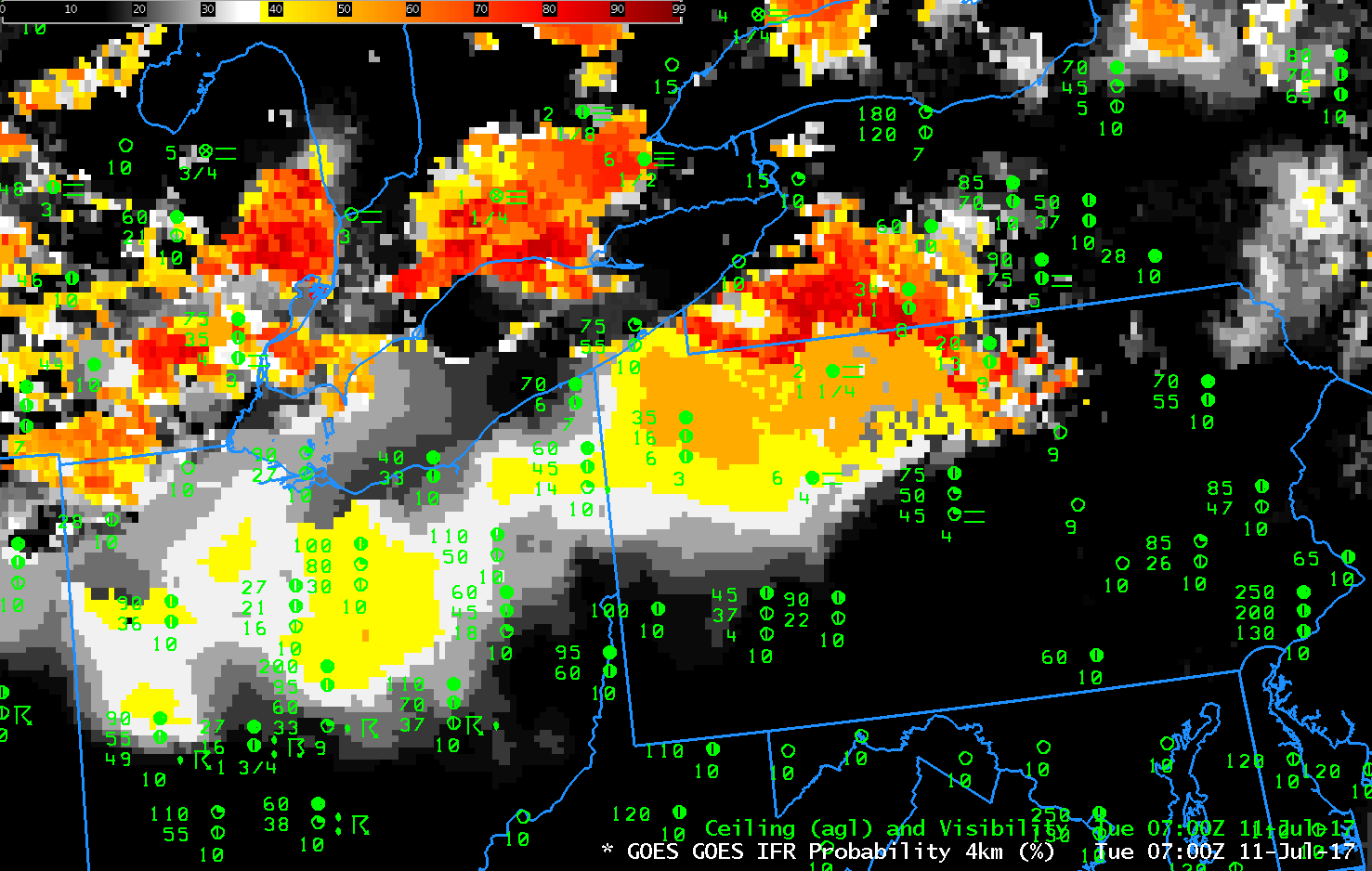
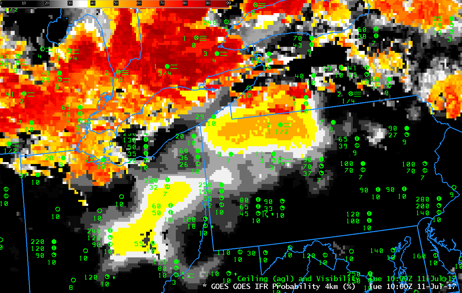
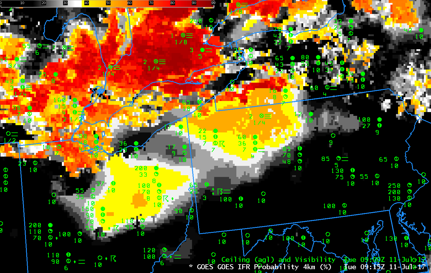
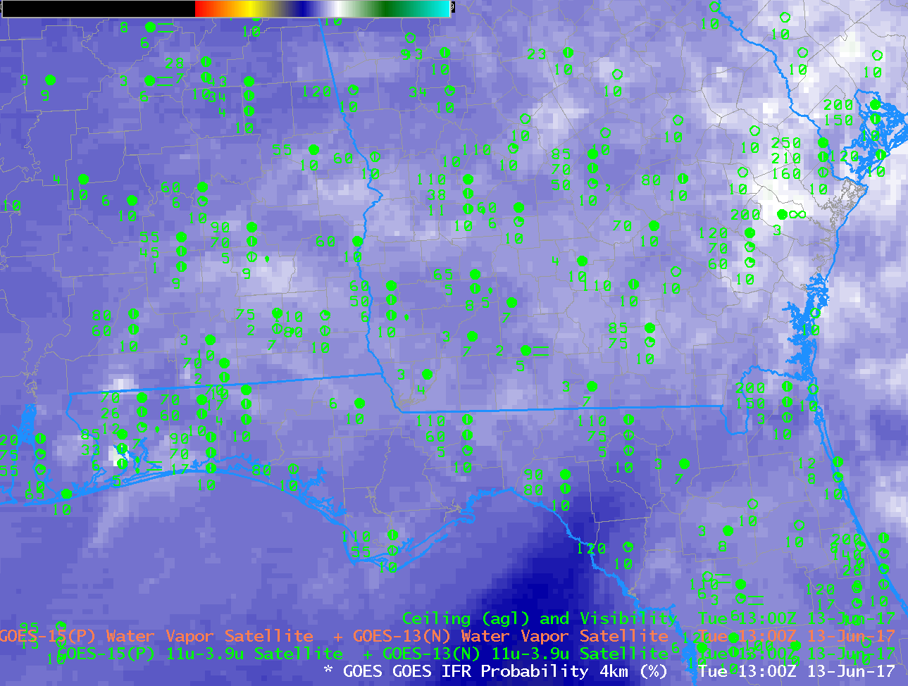
Fog and low stratus were widespread on 8 October over the Plains, in particular over Iowa and Minnesota.  What satellite tools exist to highlight such regions of lowered ceilings and reduced visibility?

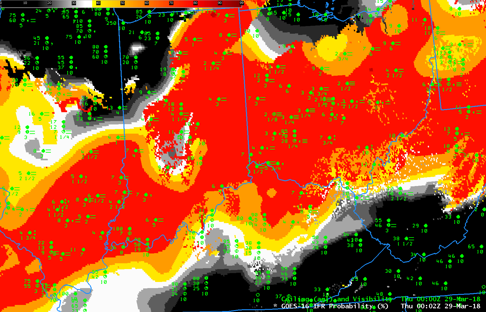
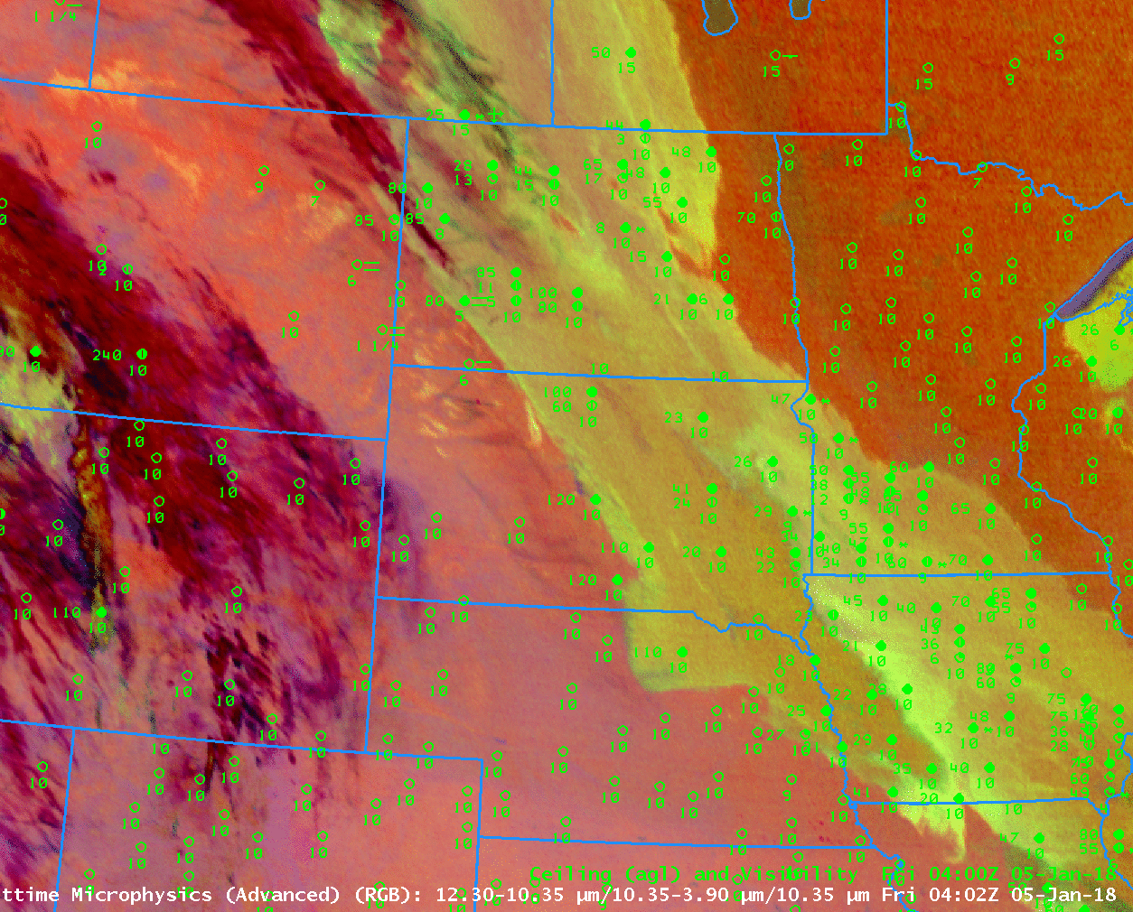
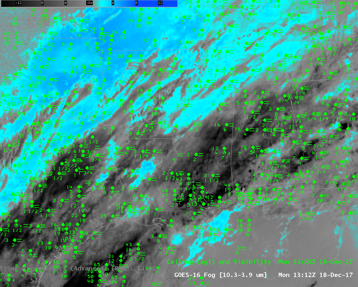
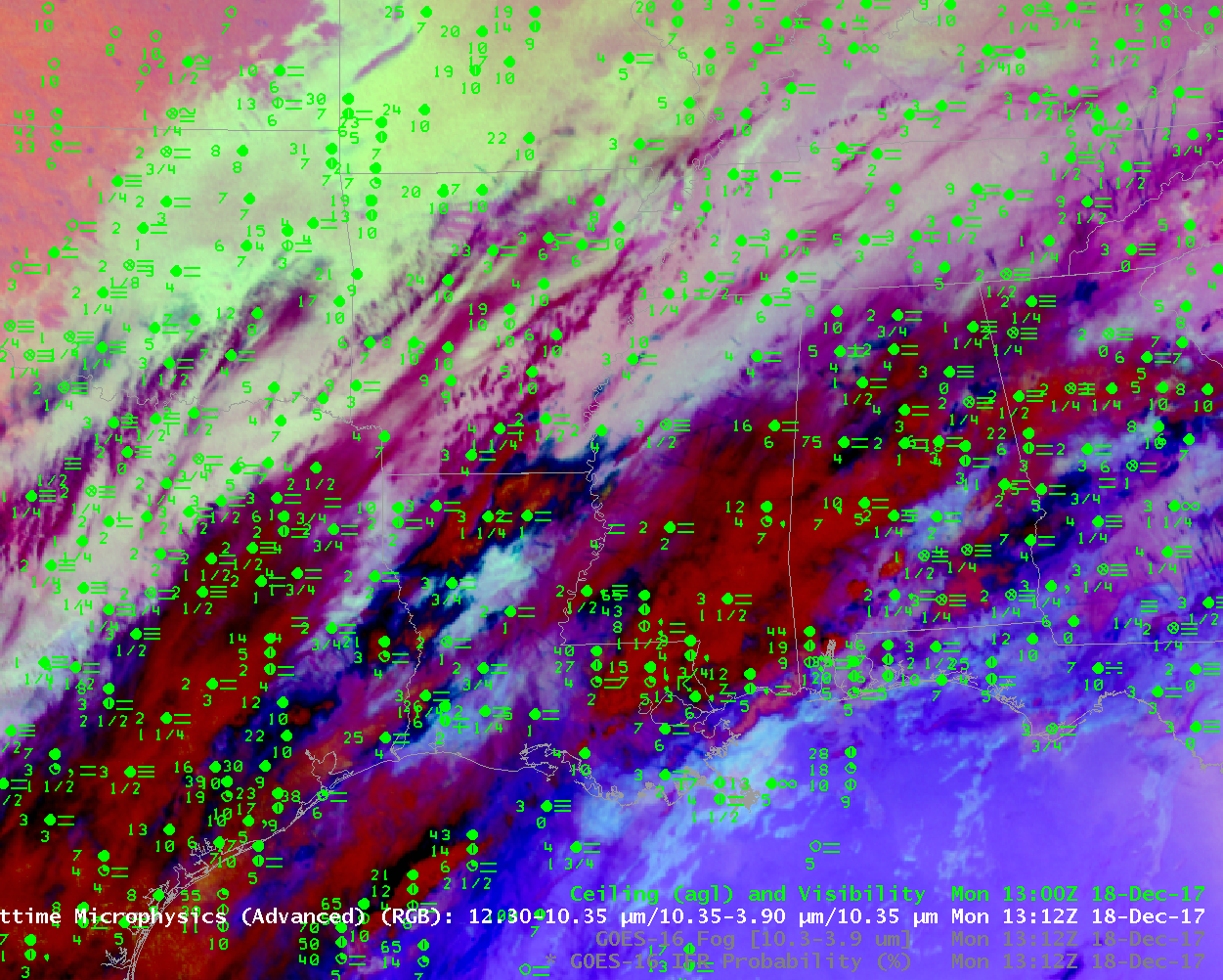
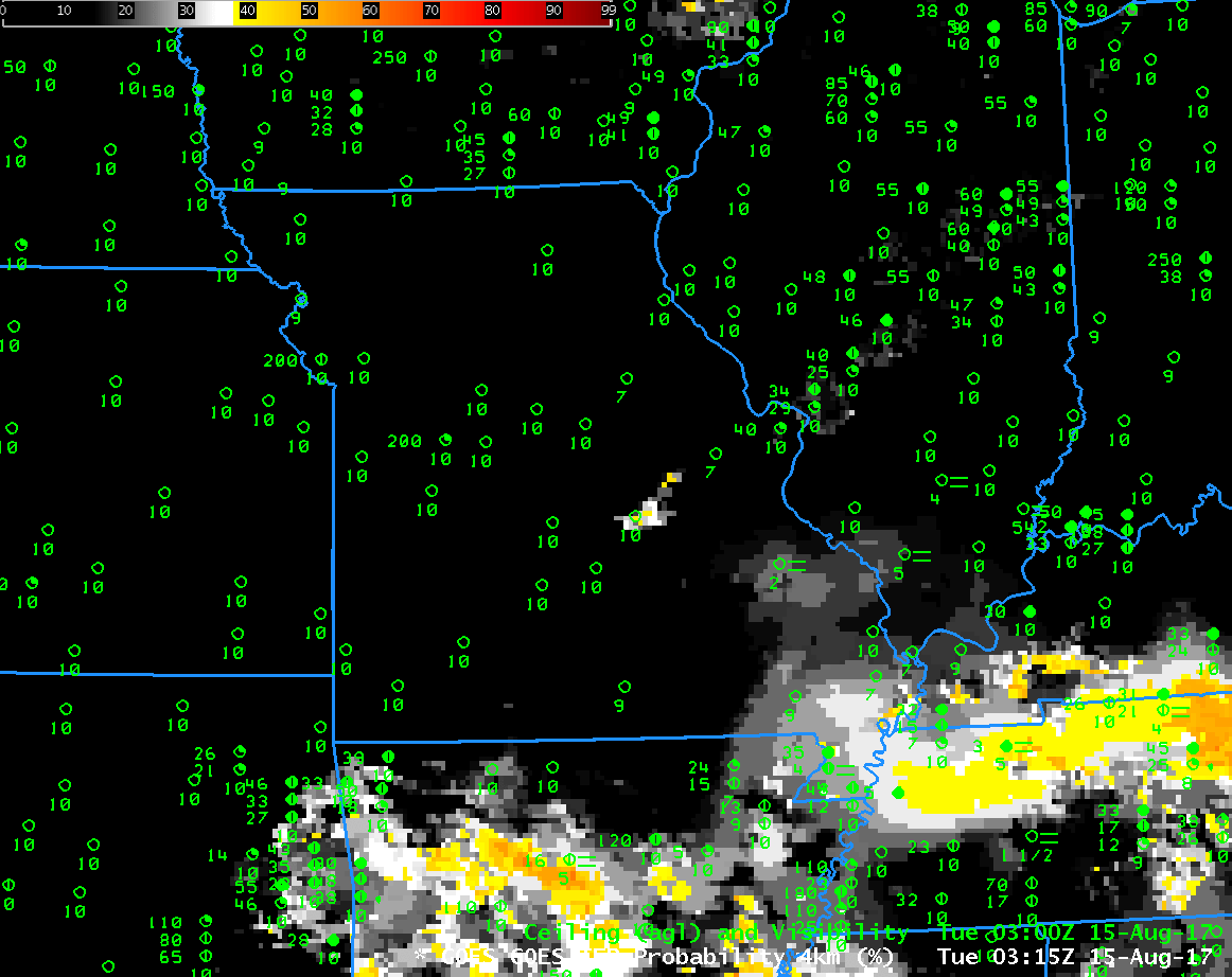
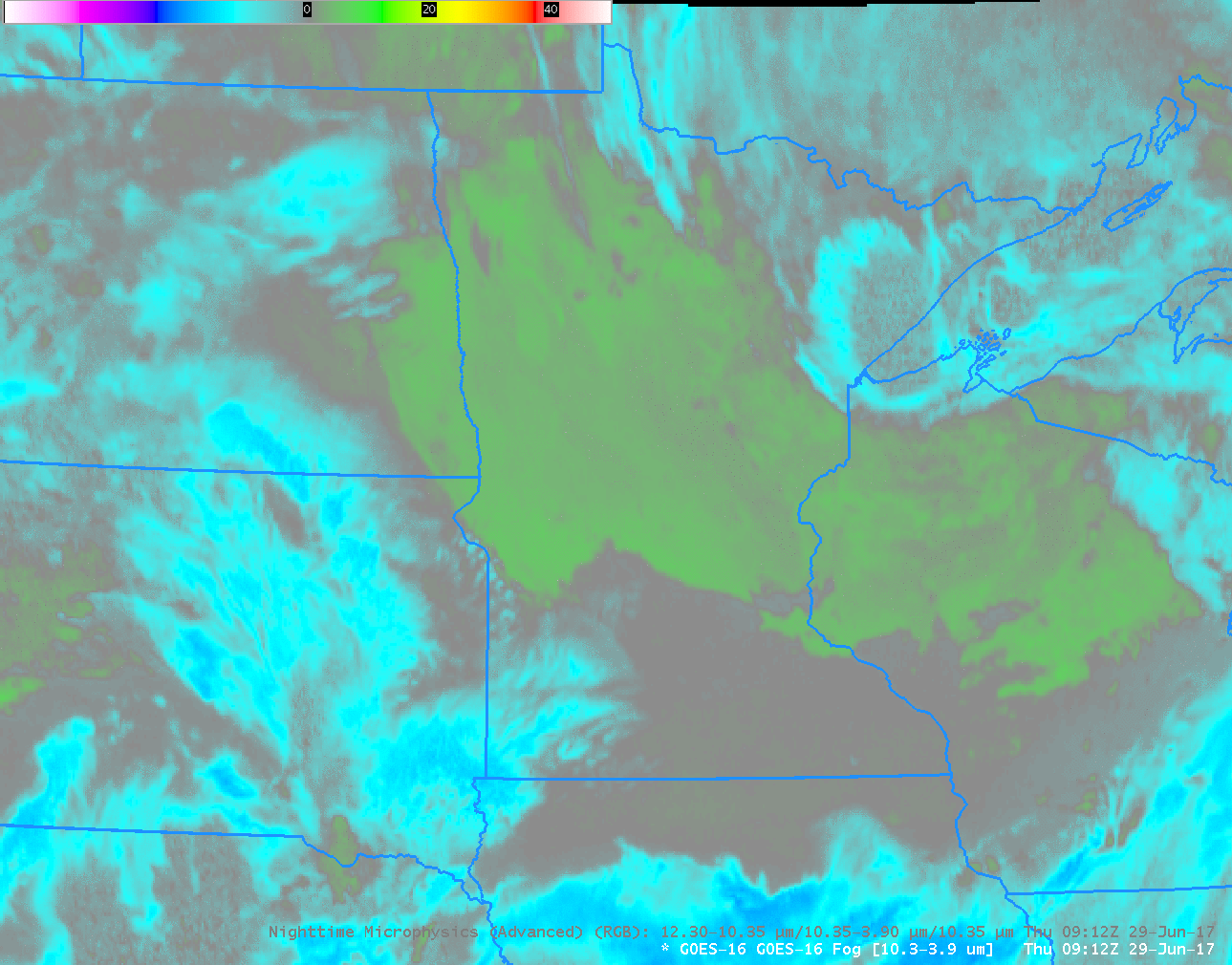
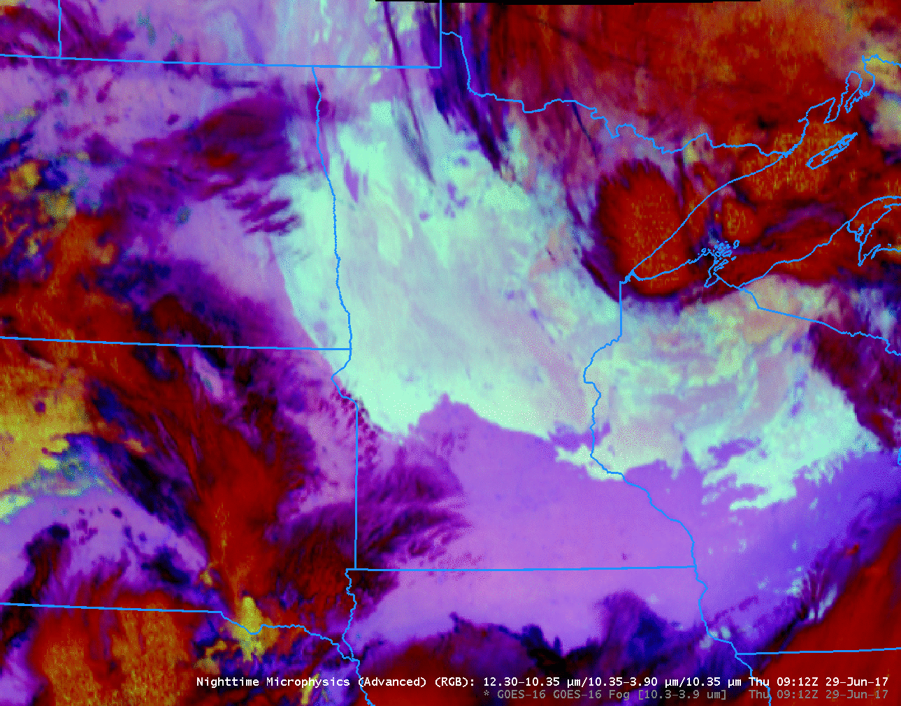
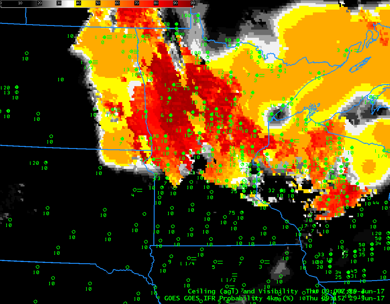
When IFR conditions — fog and low stratus — occur with extratropical cyclones that generate multiple cloud layers, satellite detection of low clouds is difficult because higher clouds get in the way of the near-surface view. The animation above steps through the Night Fog Brightness Temperature Difference (10.3 µm – 3.9 µm; low clouds in the default enhancement are cyan), the Nighttime Microphysics Red-Green_blue (RGB) composite (low clouds in the RGB are cyan to yellow, depending on the temperature) and the GOES-R IFR Probability field (Probabilities for IFR conditions are highest in orange/red regions) for 1142 UTC on 8 October 2018, when low ceilings were widespread over the Plains and East Coast. Abundant high clouds rendered the Night Fog Brightness Temperature difference product (and, by extenstion, the Night Time Microphysics RGB, because the RGB uses the Night Fog Brightness Temperature Difference as its ‘Green’ Component) ineffective in outlining potential regions of low clouds. In contrast, the IFR Probability field was able to highlight low clouds under the high clouds because it fuses satellite data (ineffective at this time) with Rapid Refresh model estimates of low-level saturation.

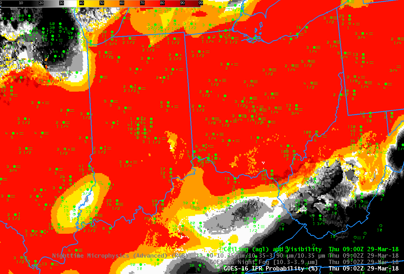
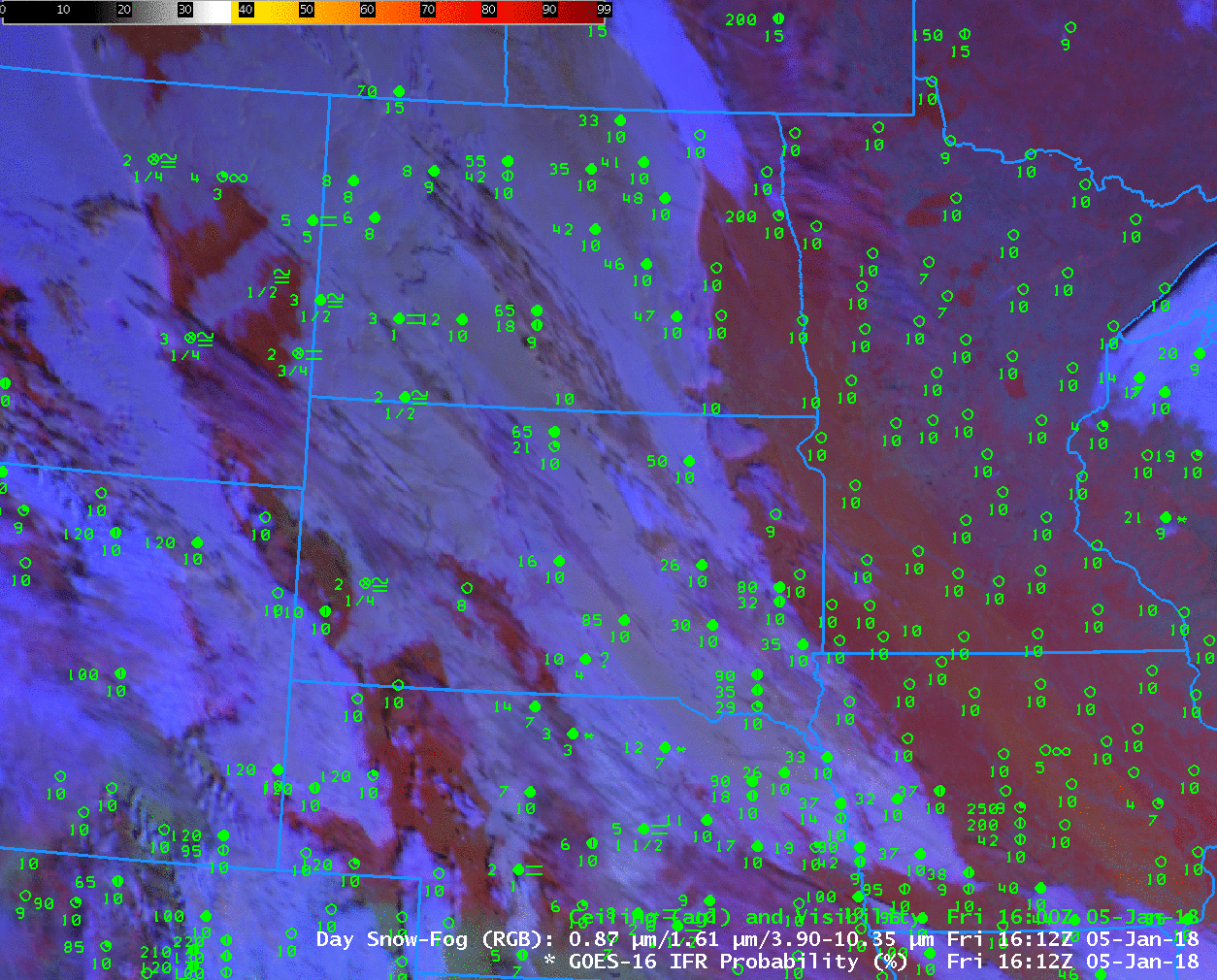
There are regions — southern Lake Erie, for example — where the lack of high clouds allows the Brightness Temperature Difference field, and the Nighttime Microphysics RGB to operate with success in identifying low clouds.

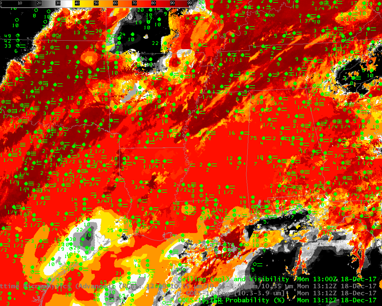
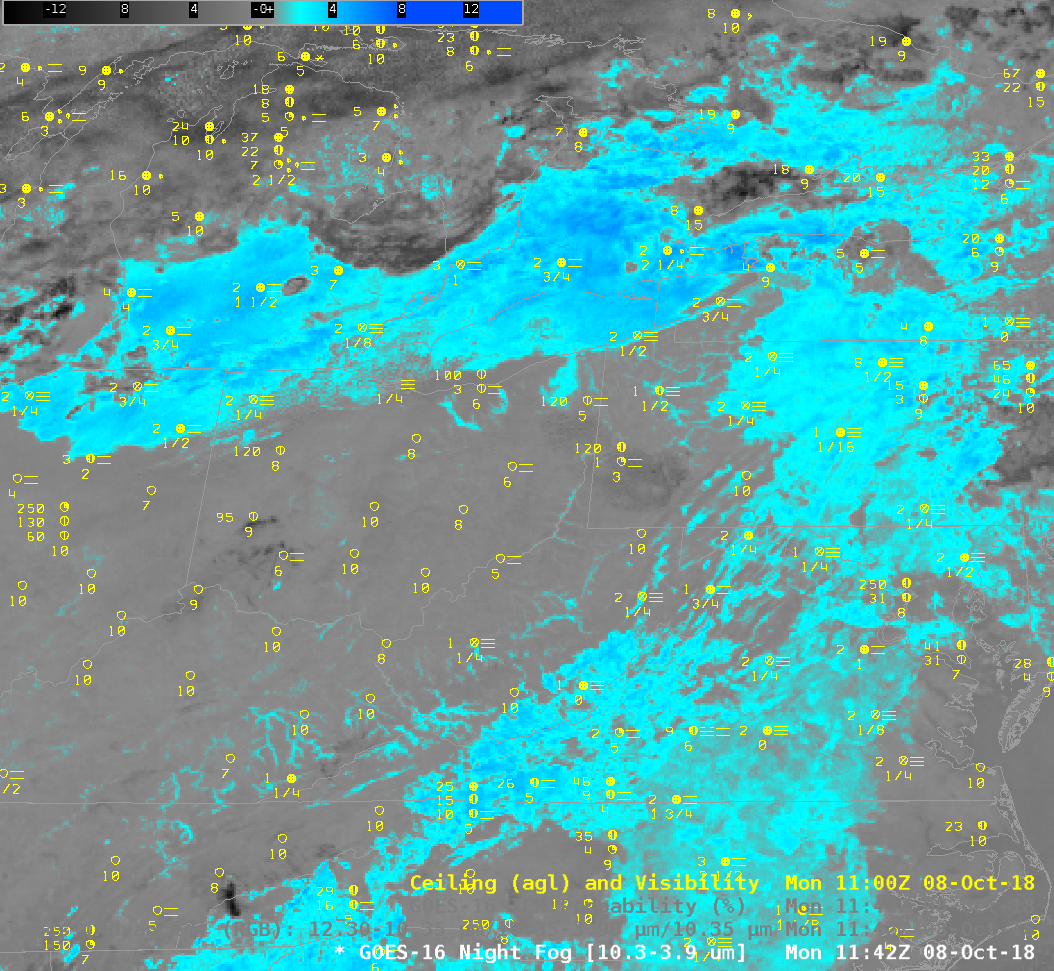
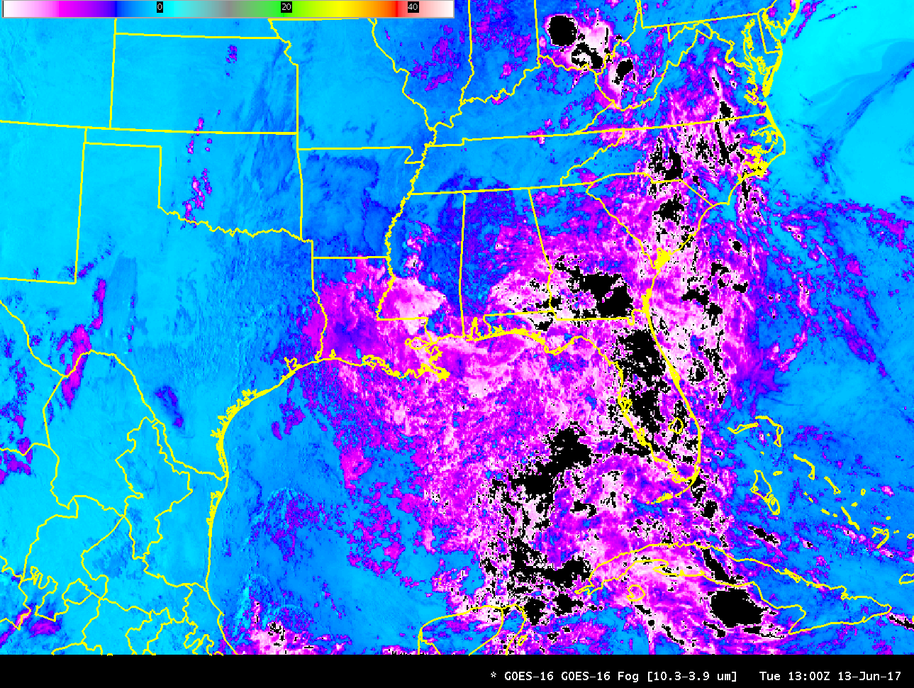
The toggle below shows the Night Fog Brightness Temperature Difference and the IFR Probabiity fields over the eastern portion of the country.  Very small-scale (in the horizontal) features, such as river fog, are a challenge for IFR probability because the Rapid Refresh horizontal resolution of 13 km may not resolve river valleys.

GOES-16 Night Fog Brightness Temperature Difference (10.3 µm – 3.9 µm) and GOES-16 IFR Probability fieds at 1142 UTC on 8 October 2018 (Click to enlarge)

Advection Fog with a Spring Storm in the Ohio River Valley

GOES-16 IFR Probability fields, 0002 UTC through 1152 UTC on 29 March 2018, every 20 minutes (Click to enlarge)

Advection fog in the Spring, when high dewpoints overrun very cold ground surfaces, usually in association with an extratropical cyclone, are very difficult to detect using satellite-only products, as shown in the Brightness Temperature Difference field animation below (Click here for the same animation but with a 5-minute time step as observed in the CONUS domain by GOES-16). GOES-16 IFR Probability, above (Click here for an animation with a 5-minute cadence), is able to highlight the region of low ceilings and visibilities because Rapid Refresh Data supplies information about near-surface saturation that is lacking in satellite-only products such as the Brightness Temperature Difference, below, or, say, the Nighttime Microphysics RGB that uses the Brightness Temperature Difference. A toggle including IFR Probability, Night Fog Brightness Temperature Difference, and Nighttime Microphysics is below (from 0902 UTC on 29 March). Only the IFR Probability has an obvious signal difference between regions with IFR Conditions and regions without.

GOES-16 Night Fog Brightness Temperature Difference (10.3 µm – 3.9 µm), 0002 – 1152 UTC at 20-minute timesteps (Click to enlarge)

GOES-16 IFR Probability, Night Fog Brightness Temperature Difference (10.3 µm – 3.9 µm), and Nighttime Microphysics at 0902 on 29 MArch 2018 (Click to enlarge)

IFR Probability discriminates between fog and elevated stratus over Texas

GOES-16 IFR Probability field, 1127 UTC on 13 February, along with observations of ceilings and visibility. (Click to enlarge)

GOES-16 IFR Probability fields on 13 February at 1127 UTC, above, suggest a clear difference in sky conditions between northeast Texas, where IFR Probabilities are very high, and where IFR conditions are widespread, and north-central Texas, around Dallas, where IFR Probabilities are small, and where ceilings and visibilities do not match IFR Conditions.

In contrast, the Brightness Temperature Difference field, below, (and the Nighttime Microphysics Red/Green/Blue product, shown here in a toggle with the Brightness Temperature Difference field) shows little difference in signal between the region of IFR conditions over northeast Texas and non-IFR conditions over Dallas and environs.

GOES-16 views the top of the cloud, and a region of fog and a region of stratus can look very similar in the Night Fog Brightness Temperature Difference. Because IFR Probability fields fuse satellite observations of low clouds with Numerical Model Output estimates of near-surface saturation, IFR Probabilities can differentiate between regions of elevated stratus (where near-surface saturation is not suggested by the model), such as near Dallas, and regions of stratus that is obstructing visibility (where near-surface saturation is suggested by the model).

A toggle of all three fields is shown at the bottom of this post.

GOES-16 Night Fog Brightness Temperature Difference (10.3 µm – 3.9 µm), 1127 UTC on 13 February 2018 (Click to enlarge)

GOES-16 IFR Probabilities, Night Fog Brightness Temperature Difference (10.3 µm – 3.9 µm) and NightTime Advanced Microphysics RGB, 1127 UTC on 13 February 2018 (Click to enlarge)

Advection Fog with a strong storm in the Midwest

GOES-16 IFR Probabilities, 1152 UTC on 22 January 2018, along with 1200 UTC surface observations of ceilings and visibilities (Click to enlarge)

When skies are clear, and radiation fog forms, limiting visibilities, it’s straightforward to use satellite-only products to gauge where stratus and fog might exist. Extratropical storms generate multiple cloud layers, however; when warm sector air under multiple cloud layers overruns snow-covered or frozen ground, dense advection fog can develop, and that fog is difficult to discern from satellite because it is typically overlain by higher clouds.

GOES-R IFR Probabilities, above, (and Low IFR Probabilities here) show highest probabilities in general occur in the regions where IFR conditions were observed on 22 January.  Over much of Wisconsin and Minnesota, the IFR Probability field is mostly uniform.  Such a flat field is characteristic of a region where satellite data cannot be used to judge whether low stratus is present (because high clouds are also present).  Rapid Refresh model information only is used to outline regions of low-level saturation. There is more variability to the IFR Probability field — that is, it is more pixelated — over southwest Iowa, for example, and over North Dakota.  In these regions, low stratus clouds are being observed by satellite and both satellite and model data can be used to estimate regions of significantly reduced ceilings and visibilities.

Consider the Brightness Temperature Difference shown below. The 10.3 µm – 3.9 µm product is typically used to identify stratus and radiation fog, and it does detect those low clouds over North Dakota, and over Kansas, Missouri and southern Iowa, and over Ontario.  However, the dense clouds associated with the storm over much of Minnesota and Wisconsin meant that this brightness temperature difference field, and also the NightTime Microphysics Red Green Blue Product (which is sometimes used to detect fog), could not ‘see’ the fog over the upper midwest.

Know the limitations, strengths and weaknesses of your products as you use them!  On 22 January, High Clouds underscored limitations in the Brightness Temperature Difference product, and in the NightTime Microphysics product that relies on the Brightness Tempearature Difference product for fog detection.  That limitation meant the product was not useful in identifying IFR conditions in parts of the Upper Midwest.

GOES-16 “Night Fog” Brightness Temperature Difference (10.3 µm – 3.9 µm) at 1152 UTC on 22 January 2018. Surface reports of ceilings and visibilities at 1200 UTC are also plotted (Click to enlarge)

Dense Fog Advisories over the Plains

Dense Fog Advisories were issued over parts of the central and northern Plains states on Friday January 5. For example, from the North Platte Office (similar warnings were issued by Billings, Rapid City and Bismark offices):

URGENT – WEATHER MESSAGE
National Weather Service North Platte NE
634 AM CST Fri Jan 5 2018

…Areas of dense fog likely this morning…

.Areas of fog reducing visibilities below one quarter mile at
times will be likely from parts of southwest into the central
Nebraska Sandhills this morning. With the fog occurring where
temperatures are below freezing, some slick spots may develop on
area roads and sidewalks as well.

NEZ025-026-037-038-059-071-051800-
/O.NEW.KLBF.FG.Y.0001.180105T1234Z-180105T1800Z/
Thomas-Blaine-Logan-Custer-Lincoln-Frontier-
Including the cities of Thedford, Halsey, Dunning, Purdum,
Brewster, Stapleton, Broken Bow, North Platte, Curtis, Eustis,
and Maywood
634 AM CST Fri Jan 5 2018

…DENSE FOG ADVISORY IN EFFECT UNTIL NOON CST TODAY…

The National Weather Service in North Platte has issued a Dense
Fog Advisory, which is in effect until noon CST today.

* Visibilities…as low as one quarter mile or less at times.

* Timing…Through the morning hours with visibilities improving
after noon CST.

* Impacts…Hazardous driving conditions due to low visibility.
Fog may freeze on area roads and walkways as well.

PRECAUTIONARY/PREPAREDNESS ACTIONS…

A Dense Fog Advisory means visibilities will frequently be
reduced to less than one quarter mile. If driving, slow down, use
your headlights, and leave plenty of distance ahead of you.

&&

$$

JWS

GOES-16 IFR Probability fields captured the development of these regions of dense fog. The animation from 0400-1200 UTC on 5 January is below. Highest values of IFR Probability are consistent in the areas where IFR Conditions are developing and where Dense Fog Advisories were issued.

GOES-16 IFR Probability, 0402 – 1207 UTC on 5 January 2018 (Click to animate)

Note that IFR Probability fields are fairly high over Iowa and the eastern Dakotas, regions where mid-level stratus was widespread but where IFR observations did not occur. On this day, Low IFR Probability fields better screened out this region of mid-level stratus. The toggle below compares IFR Probability and Low IFR Probability on 0957 UTC. The region where dense fog advisories were issued shows high values in both fields. The stratus deck over Iowa and the eastern Dakotas shows much smaller values of Low IFR Probability.

GOES-16 also has a ‘Fog Product’ brightness temperature difference (10.3 – 3.9) that has historically been used to detect low clouds. However, when cirrus clouds are present, as on 5 January, the efficacy of this product in fog detection is affected. Although fog and stratus detection is identifiable underneath the moving cirrus (the same is true in the Advanced NightTime Microphysics RGB product below), identifying the low cloud as stratus or fog from satellite data is a challenge because a consistent color married to IFR Probability does not exist.

GOES-16 ‘Fog Product’ Brightness Temperature Difference (10.3 µm – 3.9 µm), 0402 – 1207 UTC, 5 January 2017 (Click to animate)

GOES-16 Advanced Nighttime Microphysics RGB, 0402-1207 UTC on 5 January 2018 (Click to animate)

GOES-16 IFR Probability fields maintain a consistent look from night to day. Both the (10.3 µm – 3.9 µm) Brightness Temperature Difference field and the Advanced Nighttime Microphysics RGB (that uses the ‘Fog Product’ BTD) will change because the increase in reflected solar radiation at 3.9 µm will change the sign of the Brightness Temperature Difference field. There is a Daytime Day/Snow/Fog RGB Product in AWIPS, and the toggle below from 1612 UTC on 5 January compares IFR Probability and the Day/Snow/Fog RGB. As with the nighttime products, the presence of high (or mid-level) clouds makes it difficult to use the RGB alone to identify regions of fog/low stratus. In contrast, the IFR Probability field continues to correctly identify where the obstructions to visibility exist.

Dense Fog over the Deep South

GOES-16 IFR Probability fields, 1312 UTC on 18 December 2017 (Click to enlarge). Ceilings and visibilities are also plotted.

Dense Fog was widespread across the south on Monday morning, 18 December 2017 (See the screen capture below from this site at 1319 UTC).  The GOES-16 IFR Probability field, above, highlights the regions of IFR and near-IFR conditions very well. It has a flat character over much of central Mississippi and Alabama.  These are regions where multiple cloud decks are preventing the satellite from viewing the near-surface clouds, and where Rapid Refresh data are being used as the sole predictor for the probability of IFR conditions.  In contrast, the IFR Probability field over much of Tennessee and Arkansas (for example) has a pixelated look to it — there are small variations over very small distances:  over these two states, higher clouds are not preventing the satellite from viewing near-surface clouds, and satellite data can also be used as a predictor in the IFR Probability fields (See the 10.3 µm – 3.9 µm Brightness Temperature difference field below).

Screen Capture from http://www.weather.gov at 1319 UTC on 18 December 2017 (Click to enlarge). Grey regions are under Dense Fog Advisories.

When high clouds are present, fog detection techniques that rely solely on satellite data struggle to detect low clouds.  Compare the above field, for example, to the 10.3 µm – 3.9 µm Brightness Temperature Difference field (sometimes called the ‘Fog Product’).  In the enhancement used (the default enhancement in AWIPS), fog is depicted as blue (a positive value in the brightness temperature difference) and cirrus/high clouds in black.  There is little signal of Fog over a region where Dense Fog advisories have been issued. Similarly, the Advanced Nighttime Microphysics RGB, below, that relies on the 10.3 µm – 3.9 µm to highlight low clouds that might be fog, also is not indicating fog (a light cream/cyan color, typically) over much of the Deep South.  When cirrus clouds are present, its use, like that of the Fog Brightness Temperature Difference, is of dubious value.

The last figure, at the bottom, toggles between all three fields at 1312 UTC.

GOES-16 Fog Brightness Temperature Difference (10.3 µm – 3.9 µm) field, 1312 UTC on 18 December 2017  (Click to enlarge)

Advanced Nighttime Microphysics RGB, 1312 UTC on 18 December 2017  (Click to enlarge)

GOES-16 IFR Probability, GOES-16 ‘Fog’ Brightness Temperature Difference (10.3 µm – 3.9 µm), and Advanced Nighttime Microphysics RGB, all at 1312 UTC on 18 December 2017 (Click to enlarge)

Dense Fog over Missouri

GOES-R IFR Probability Fields, and surface reports of Ceilings and Visibilities, hourly from 0315 to 1315 UTC on 15 August 2017 (Click to enlarge)

GOES-R IFR Probabilities are computed using Legacy GOES (GOES-13 and GOES-15) and Rapid Refresh model information; GOES-16 data will be incorporated into the IFR Probability algorithm in late 2017

IFR Conditions and Dense Fog developed over southeastern Missouri during the early morning on 15 August 2017, leading to the issuance of Dense Fog Advisories. GOES-R IFR Probabilities, above, showed increasing values as the ceilings lowered and visibilities dropped.  The IFR Probability fields over southern Missouri and northern Arkansas (and Kansas and Oklahoma) have the characteristic uniformity that arises when Rapid Refresh data alone are used to drive the IFR Probability values.  In these regions, high clouds (associated with convection over Arkansas) are blocking the satellite view of lower clouds.

Such high clouds will make it difficult for a satellite-only product to identify the regions of clouds.  For example, the Brightness Temperature Difference field below (10.3 µm – 3.9 µm) from GOES-16, color-enhanced so that low clouds are green and that cirrus (at night) are purple) shows widespread low cloudiness at the start of the animation, including some obvious river fog over Missouri (river valleys that are not well-resolved with GOES-13), but developing convection over Arkansas eventually prevents the view of low clouds.

GOES-16 data posted on this page are preliminary, non-operational and are undergoing testing

GOES-16 Brightness Temperature Difference field (10.3 µm – 3.9 µm), hourly from 0312 to 1312 UTC on 15 August 2017 (Click to enlarge)

Because the Brightness Temperature Difference field (helpfully called the ‘Fog’ Channel Difference in AWIPS) is challenged by high clouds in viewing the low clouds, RGB Products that use the brightness temperature difference field are also similarly impeded by high clouds.  Consider, for example, the stations in southern Missouri shrouded by the cirrus shield.  IFR Conditions are occurring there and a strong signal of that appears in the IFR Probability fields.

GOES-R IFR Probability computed with GOES-13 and Rapid Refresh Data, GOES-16 Fog (10.3 µm – 3.9 µm) Brightness Temperature Difference and GOES-16 Advanced Nighttime Microphysics RGB, all near 1115 UTC on 15 August 2017 (Click to enlarge)

Why Fused Data is better than Satellite Data alone in detecting IFR Conditions: Pennsylvania Example

GOES-R IFR Probability Fields, 0200-1100 UTC on 11 July 2017 (Click to enlarge)

GOES-16 data posted on this page are (still!) preliminary, non-operational data and are undergoing testing

GOES-R IFR Probabilities are computed using Legacy GOES (GOES-13 and GOES-15) and Rapid Refresh model information; GOES-16 data will be incorporated into the IFR Probability algorithm in late 2017

Low ceilings and reduced visibilities developed in and around thunderstorms from Ohio and Michigan into southwestern Ontario, upstate New York and northern Pennsylvania during the morning of 11 July 2017. (Reduced visibilities/lowered ceilings persisted past 15 UTC as shown in this image from here). Regions of IFR conditions over northwestern Pennsylvania are in regions of higher IFR Probability after 0500 UTC (over northwest Pennsylvania) and after 0700 UTC (over much of northern Pennsylvania) that have the characteristic flat field look that comes from having only Rapid Refresh Model output drive the Probability (because high clouds, as might occur downwind of Convection, prevent the satellite from seeing low clouds). GOES-R IFR Probability fields also retain a signal through sunrise, as shown in the this toggle between 1000 UTC and 1100 UTC, two times on either side of the terminator.

Because high clouds inhibit the view of low stratus (and potential fog), products that rely on solely satellite data become ineffectual as a situational awareness tool. Consider the toggle below from 0800 UTC of GOES-R IFR Probabilities, the GOES-16 “Fog Product” Brightness Temperature Difference (10.3 µm – 3.9 µm) and the Advanced Nightime Microphysics RGB (that uses the Brightness Temperature Difference Product as one of its components). IFR Conditions over NW Pennsylvania are not diagnosed by the GOES-16 products that rely on the 10.3 µm – 3.9 µm Brightness Temperature Difference field. Where there is a clear field of view, all three products can highlight IFR conditions (in/around London Ontario, for example). Regions of low stratus — but not fog — are also highlighted over parts of upstate New York by the GOES-16 products. (Similar toggles at 0915 and 1100 UTC are available; note that the signal from GOES-16 becomes weak at 1102 UTC because increasing amounts of solar reflectance change the sign of the 10.3 µm – 3.9 µm Brightness Temperature Difference.

These examples typify why GOES-R IFR Probability fields typically have better statistics as far as IFR detection is concerned: Model data fills in regions where high clouds are present, and model data screens out regions where stratus is highlighted by a Brightness Temperature Difference field, but where fog does not exist.

GOES-R IFR Probabilities (computed using GOES-13 and Rapid Refresh Data), GOES-16 “Fog Product” Brightness Temperature Difference (10.3 µm – 3.9 µm) and the Advanced Nighttime Microphysics RGB, all around 0800 UTC on 11 July 2017 (Click to enlarge)


Methods of Fog Detection in the GOES-16 Era

GOES-16 ‘Fog Detection’ Channel Difference (10.3 µm – 3.9 µm), 0912 – 1132 UTC, 29 June 2017 (Click to enlarge)

GOES-16 data posted on this page are (still!) preliminary, non-operational data and are undergoing testing

The 16 channels on the GOES-R Series Advanced Baseline Imager (ABI) allow for many different channel combinations that can be used to detect atmospheric phenomena. The animation above shows the traditional method for detecting low stratus: the brightness temperature difference between the shortwave infrared (3.9 µm) and the cleanest longwave infrared (10.3 µm) windows. Cloudtops composed of water droplets are highlighted in the animation because they do not emit 3.9 µm radiation as a blackbody, but do emit 10.3 µm radiation as a blackbody; thus, the brightness temperature difference at night (when no reflected solar radiation at 3.9 µm is present) is positive. The range of the colorbar in the above animation is from -50 to +50 C; stratus appears as green over much of northern Wisconsin, Minnesota and North Dakota.  Higher cirrus clouds are cyan, and they interfere with the satellite detection of low clouds, especially over eastern North Dakota where IFR conditions were widespread (source), and where a Dense Fog Advisory existed.  Note the apparent disappearance of the fog signal — in green — as the sun rises.  Increasing amounts of reflected solar radiation are causing the brightness temperature difference value to switch sign from (10.3 µm – 3.9 µm) > 0 at night (because of emissivity differences) to (10.3 µm – 3.9 µm) < 0 during the day (because of solar reflectance).

The ‘Nighttime Microphysics Advanced RGB’ is also used as a fog detection device. In the animation below, low stratus (and by inference, fog) is highlighted in cyan, a signal that comes mostly from the ‘green’ part of the RGB, namely the Brightness Temperature Difference as shown above. Because the two products are linked by the 10.3 – 3.9 brightness temperature difference, shortcomings in that product as far as fog detection affect the RGB. Note how the fog signal erodes over Minnesota/Wisconsin as the sun rises, and how it is obscured by high clouds (dark purple/magenta) over North Dakota.


Note: GOES-R IFR Probabilities are computed using Legacy GOES (GOES-13 and GOES-15) and Rapid Refresh model information; GOES-16 data will be incorporated into the IFR Probability algorithm in late 2017

GOES-R IFR Probability fields, shown for this event below, were designed to mitigate detection issues noted above.  Where high clouds are present, meaning the satellite cannot detect low clouds, information about low-level saturation from the Rapid Refresh is used to assess whether or not fog is likely.    That low-level information from the model also can be used to distinguish between fog and elevated stratus that can look very similar from the top, as a satellite views it.  The fusing of model and satellite data makes for a product that has better statistics in detecting low ceilings and reduced visibilities.

At the end of the two animations above, for example, how confident will a satellite analyst or forecaster be that there is dense fog over eastern North Dakota?  How about the analyst/forecaster using IFR Probability fields? IFR Probabilities maintain a signal for fog over the entire region from North Dakota to Wisconsin, even through sunrise and under high clouds.

GOES-R IFR Probabilities, 0915 to 1115 UTC on 29 June 2017 (Click to enlarge)

Fog Detection Methods when Cirrus Clouds are present

GOES-R IFR Probability fields, 0545, 0800, 1000 and 1300 UTC on 13 June 2017 (Click to enlarge)

GOES-16 data posted on this page are (still!) preliminary, non-operational data and are undergoing testing

Note: GOES-R IFR Probabilities are computed using Legacy GOES (GOES-13 and GOES-15) and Rapid Refresh model information; GOES-16 data will be incorporated into the IFR Probability algorithm in late 2017

Reduced visibilities and lowered ceilings — IFR and Low IFR conditions — occurred over a wide stretch of the southeastern United States on the morning of 13 June 2017.  The animation above shows enhanced IFR Probabilities aligned northwest to southeast from central Alabama to northwest Florida, the region where IFR Conditions develop.  The flat nature of the field suggests that satellite data are not widely available as a predictor for low clouds on this morning, and that is because of widespread cirrus clouds over the southeastern United States (Click here to see the 0545 and 1300 UTC GOES-13 Water Vapor Imagery with cold brightness temperatures over the southeast).  When high clouds are present, satellite-only detection of low clouds is not feasible.

For example, the brightness temperature difference field from GOES-13 (3.9 µm – 10.7 µm), below, has little predictive value for the northwest-to-southeast-oriented feature of low clouds/reduced visibilities because cirrus clouds are blocking the view.

GOES-13 Brightness Temperature Difference (3.9 µm – 10.7 µm) at 0545, 0800, 1000 and 1315 UTC on 13 June 2017 (Click to enlarge)

Various other detection techniques that rely on only satellite data similarly will be challenged by the presence of high clouds. For example, the Nighttime Microphysics RGB (From this site) shows little signal of fog (cyan/white in the RGB composite) over Georgia and Florida. Intermittent signals will appear occaionally as high clouds thin to allow the low-cloud signal through. The GOES-16 Brightness Temperature Difference field (10.33 µm – 3.9 µm) similarly is challenged by the presence of high clouds. The example shown at 1300 UTC shows a negative value because of reflectance off of high clouds.

Because the IFR Probability fields include surface information in the form of output from the Rapid Refresh model (saturation in the lowest part of the model is used as a predictor for the presence of fog), IFR Probability fields can fill in regions where satellite data cannot be used to detect low clouds because of the presence of high clouds. In regions where high clouds are present, satellite-only detection of fog and low stratus will always be a challenge.