Category Archives: Wisconsin

IFR Conditions during a Weak weather event

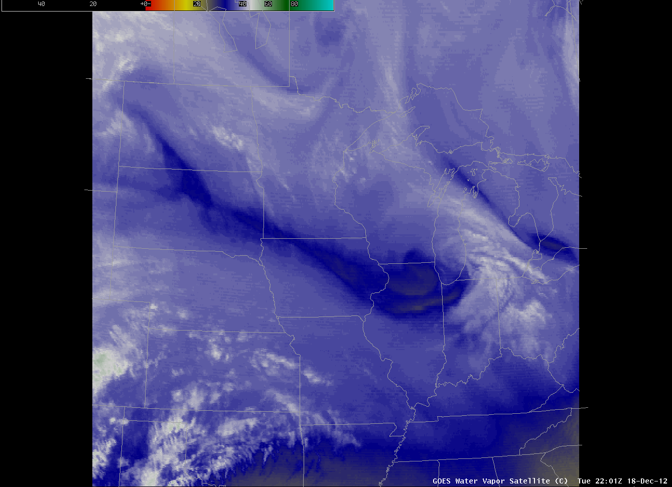
GOES-East Water Vapor Imagery (6.7 ) from 2202 UTC on 18 December 2012

A weak weather system moved through the upper Midwest on December 18th, laying down a light strip of snow over Iowa and southern Wisconsin.  The Water Vapor imagery, above, shows the small scale vorticity center that helped to force the precipitation band moving over southern Lake Michigan after most of the snow in Wisconsin had tapered off.

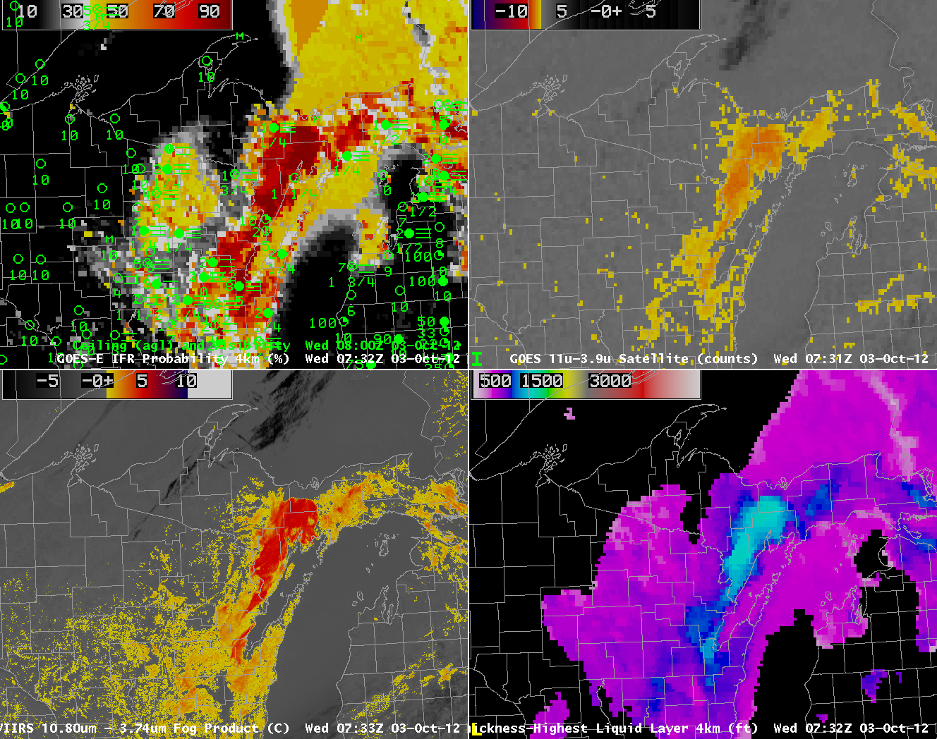
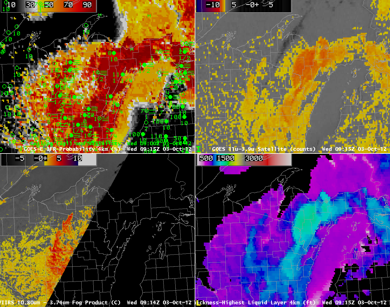
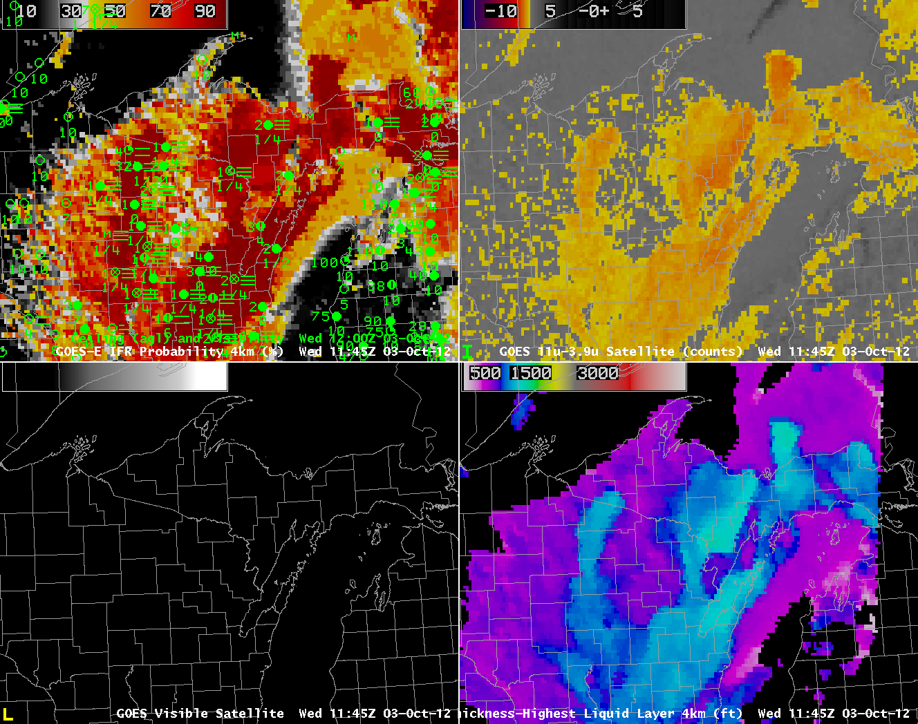
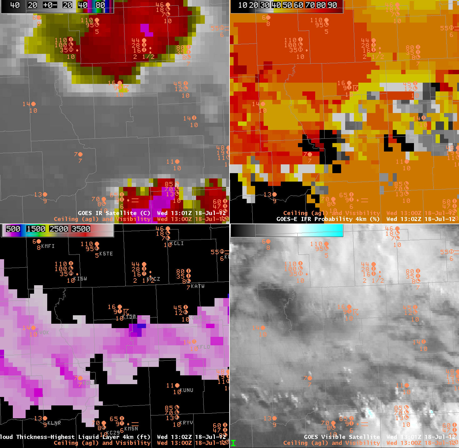
The storm left behind abundant low-level moisture, and Fog/Low Stratus that caused IFR conditions were common.  The animation of the GOES-R IFR Probability product, below, shows high probabilities in the region where light snow and drizzle persisted.  Several aspects of this image require comment.

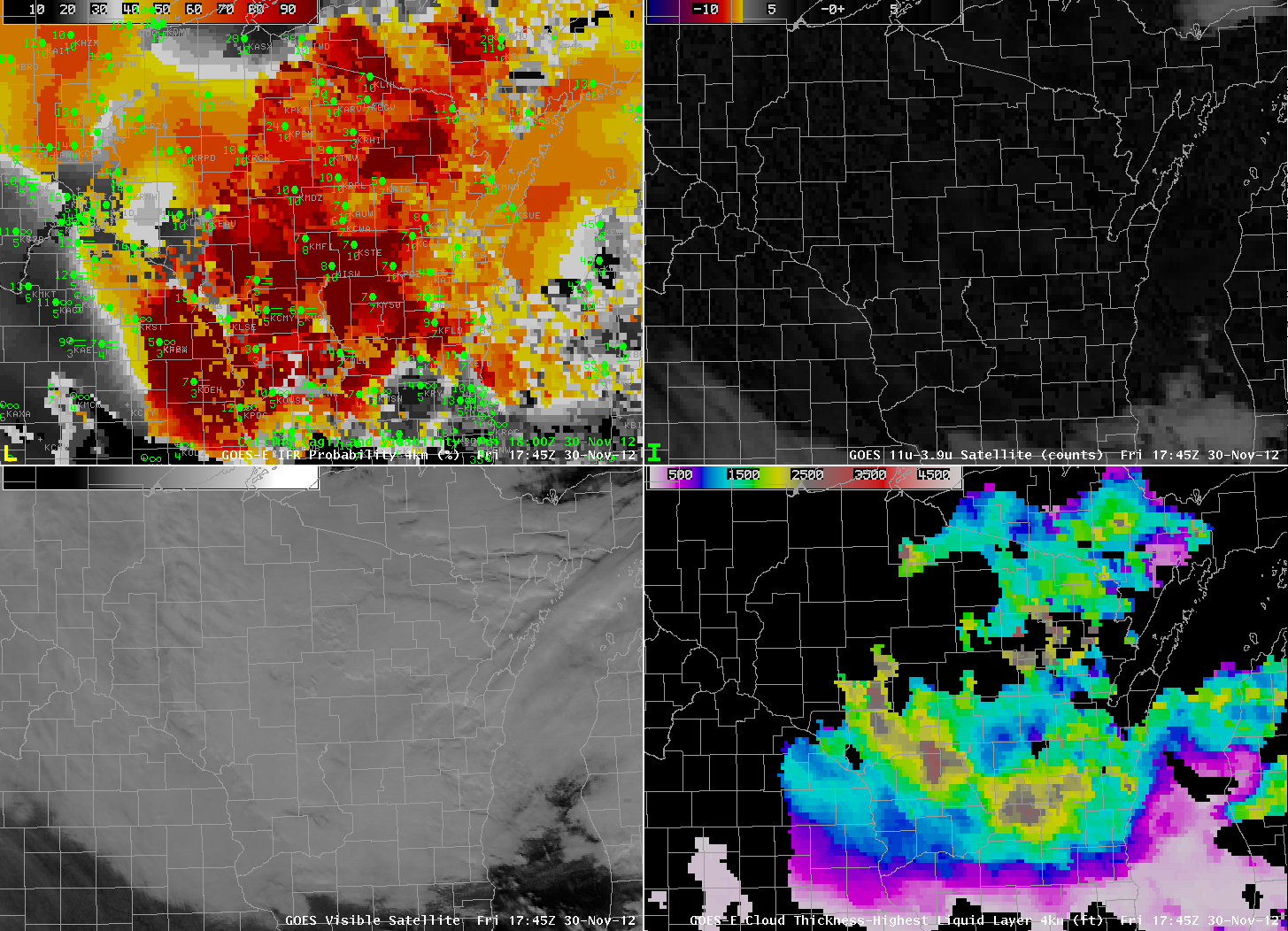
GOES-R IFR probabiltiies computed from GOES-East, and surface observations of ceilings and visibility, hourly from 2100 UTC 18 December to 0200 UTC 19 December.

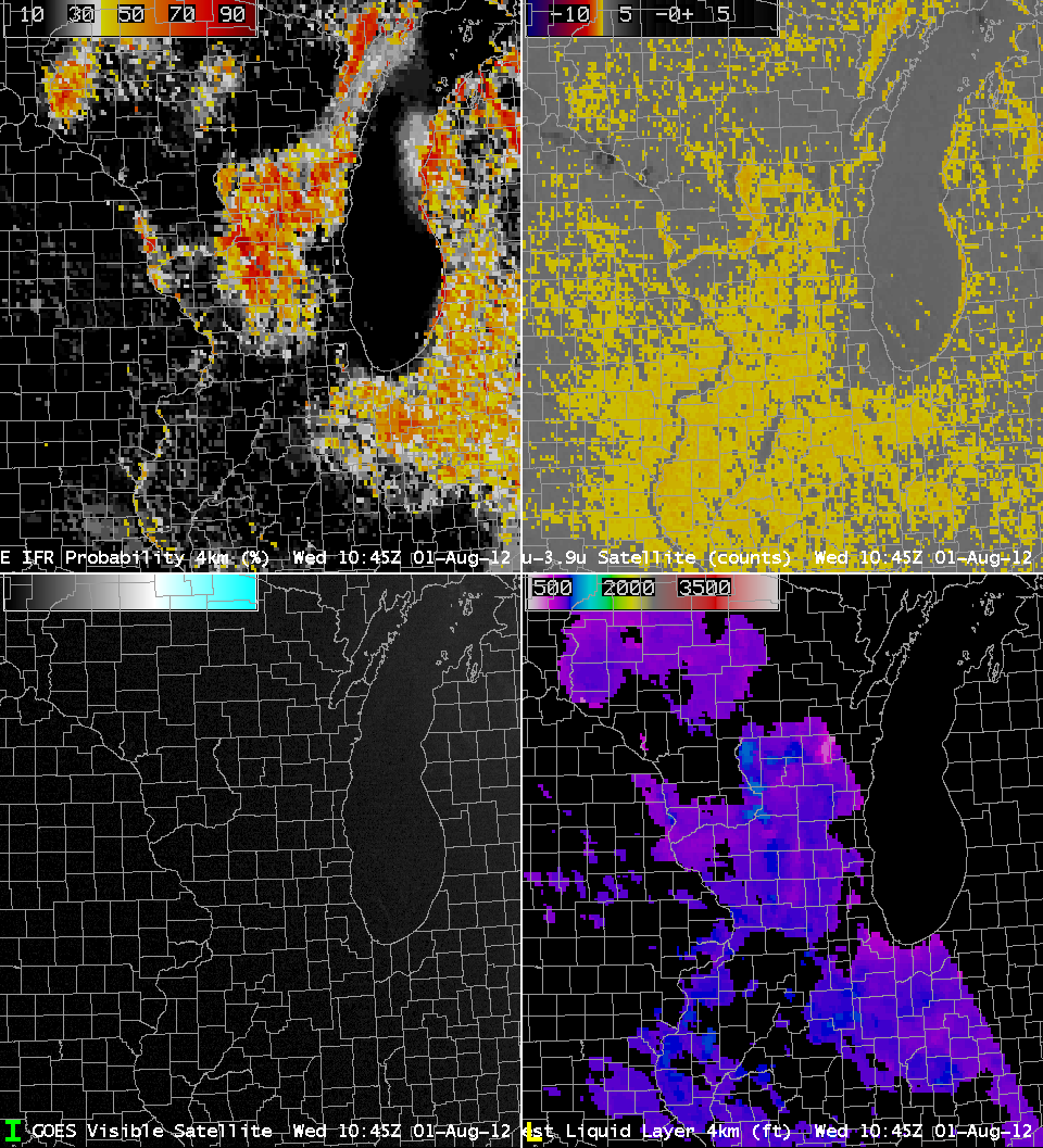
The image at 2200 UTC shows the boundary between day-time predictor use and night-time predictor use.  This boundary runs southeast to northwest over Iowa.  IFR probabilities are somewhat lower where the night-time predictors are used initially, but patches of higher IFR probability do occur.  The IFR Probability product does distinguish well between the fog and low stratus that does restrict visibility and the elevated stratus over Illinois that is obvious in the traditional brightness temperature difference product, below.  Note especially how Chicago’s O’Hare airport is not reporting IFR conditions, nor under a region where GOES-R IFR probabilities are high, but it is in a region where the traditional brightness temperature product has a strong signal.

Toggle between GOES-R IFR Probability field and GOES-East Brightness Temperature Difference Field, 0200 UTC 19 December 2012

Stratus vs Fog

GOES-R IFR Probabilties over Wisconsin, computed from GOES-East (Upper left), GOES-East brightness temperature difference (10.7 µm – 3.9 µm) (Upper right), GOES-East Visible imagery (0.62 µm) (Lower left), GOES-R Cloud thickness (Lower right)

Stratus and fog look very similar from the satellite’s perspective, both during the day and at night.  That is why it is important to include surface information in a product that detects fog and low stratus.  The IFR Probability product over stratus-bound Wisconsin at mid-day on November 30 2012 shows a diagonal stripe of higher probabilities from southwestern Wisconsin to north-central Wisconsin.  Airports that are reporting IFR or near-IFR conditions are located within this stripe.  Over the rest of the state, where IFR probabilities are lower, the large majority of airports are reporting visibilities and ceilings exceeding IFR limitations.  The character of the visibile satellite data, and of the brightness temperature difference product, gives very little indication that surface visibilities are reduced primarily from northeast Iowa/southwest Wisconsin to north-central Wisconsin.

Advection/Radiation fog over the Upper Midwest

GOES-R IFR Probabilities at 0100, 0400 and 0800 UTC on 24 October 2012

Dewpoints in the low 60s (Fahrenheit) surging into the upper Midwest in late October heighten the chances of fog, and the GOES-R Fog/Low Stratus product did a commendable job of showing where the fog might be occurring.  The loop above shows the IFR Probabilities over Wisconsin, Iowa and Minnesota as well as visibility/ceiling observations.  The northwest-southeast edge of higher probabilities over southern to west-central Wisconsin at 0100 UTC matches the observations well:  IFR conditions prevail in regions north and east of that line.  Note also, at 0400 UTC, the skinny region of enhanced IFR probabilities that hugs the western shore of Lake Michigan.  Lake Michigan lake surface temperatures are in the low 40s, so dewpoints above 50 will result in a dense advection fog.  Heightened probabilities continue at 0800 UTC over northern and eastern Wisconsin, in agreement with observations.

Heritage Fog Detection, brightness temperature difference, at 0100, 0400 and 0800 UTC on 24 October

The Brightness temperature difference field historically has been used to diagnose the presence of low clouds, and the animation above shows the importance of using fused products — that include some kind of influence from surface observations as occurs in the Rapid Refresh — to clarify exactly where the low clouds that obstruct visibility are common.  Consider the field at 0100 UTC.  The IFR probability delineates between higher visibility over southern/western Wisconsin and lower visibilities north and east.  No such delineation occurs in the tradiational product because the brightness temperature difference alone cannot indicate the ceiling.

MODIS data is also used to create IFR Probability fields, and the 0417 UTC imagery is shown below.

MODIS-based GOES-R IFR Probabilities, 0417 UTC 24 October.

FLS detection over the upper midwest

0730 UTC GOES-R IFR Probabilities computed from GOES-14 (Upper left), Traditional Brightness Temperature difference (10.7 µm – 3.9 µm) from GOES-14 (Upper Right), Brightness Temperature Difference (11.35 µm – 3.74 µm) from VIIRS on Suomi/NPP (Lower left),  Thickness of highest Liquid Water Cloud Layer (Lower Right)

Low cloud formation over northern and northeastern Wisconsin early in the morning of October 3rd 2012 demonstrated some strengths of the fused GOES-R Fog/Low Stratus product.  Note that the 0732 UTC GOES-R IFR Probability has a pocket of higher probabilityes over north-central Wisconsin (near Vilas and Oneida Counties) in a region where the traditional brightness temperature difference has a weak signal, and in a region where surface observations indicate fog is present. This region is a good example of how the model RH data can amplify weak satellite signals where fog/low clouds are present but the satellite signal alone may not be strong enough to detect it.

0915 UTC GOES-R IFR Probabilities computed from GOES-14 (Upper left), Traditional Brightness Temperature difference (10.7 µm – 3.9 µm) from GOES-14 (Upper Right), Brightness Temperature Difference (11.35 µm – 3.74 µm) from VIIRS on Suomi/NPP (Lower left),  Thickness Of highest Liquid Water Cloud Layer (Lower Right)

At 0915 UTC, the region of IFR conditions in north-central Wisconsin persists.  At this time, however, the satellite signal also increases showing a signature consistent with low clouds/fog, and therefore GOES-R IFR probabilities significantly increase.  Two things should be clear.  First, the GOES-R IFR probability predicted the presence of Fog/Low Stratus before satellite signal was strong enough to detect it alone (a benefit of using a fused data product) and could be used better to nowcast the evolving boundary layer.  Second,  GOES-R IFR Probabilities when the model signal (in this case, the Rapid Refresh) is strong and the satellite signal is weak are lower than when both model and satellite signals are strong.  This is always the case.

1145 UTC GOES-R IFR Probabilities computed from GOES-14 (Upper left), Traditional Brightness Temperature difference (10.7 µm – 3.9 µm) from GOES-14 (Upper Right), Visible Imagery (0.62 µm) from GOES-14 (Lower left),  Thickness Of highest Liquid Water Cloud Layer (Lower Right)

The 1145 UTC shows the last pre-dawn estimate of Cloud Thickness over north-central Wisconsin (the terminator is apparent, running north-south through the Straits of Mackinac).  Estimated cloud thickesses over Vilas and Oneida counties are between 1000 and 1150 feet, vs. 1250 feet over Green Bay and more than 1300 feet over southern Upper Michigan.  Predictably, then, the fog/low stratus over north-central Wisconsin dissipates before the fog/low stratus over northeast Wisconsin and eastern Upper Michigan (see below).

1602 UTC GOES-R IFR Probabilities computed from GOES-14 (Upper left), Traditional Brightness Temperature difference (10.7 µm – 3.9 µm) from GOES-14 (Upper Right), Visible Imagery (0.62 µm) from GOES-14 (Lower left),  Thickness Of highest Liquid Water Cloud Layer (Lower Right)

Satellite and Model Predictors of Fog

GOES-R IFR Probabilities (Upper left), Enhanced GOES-East 10.7 micrometer imagery (Upper right), Rapid Refresh Mean Relative Humidity (1000-850 mb) (Lower left), Composite Radar Reflectivity (Lower right).  Times as indicated.

A large convective system moved over Wisconsin during the morning of 16 August 2012 and it illustrates the importance of fused data in diagnosing IFR conditions.  The deep convective cloud precludes any satellite detection of low water-based clouds, so the traditional method of detecting fog/low stratus (the brightness temperature difference between 10.7 and 3.9 micrometers) cannot be used.  In this case, model data, in the form of Rapid Refresh Relative Humidity, is used to fill in regions where satellite predictors cannot help.  Note the observation of IFR conditions at Wisconsin Rapids (KISW);  this is a region of very high model relative humidity.  Model relative humidity is just as high over south-central Minnesota;  in that region, however, satellite predictors do exist, and they do not suggest fog/low clouds, so the IFR probability there is comparitively lower.

The character of the IFR probability field is much less pixelated in regions where model data only are used as predictors.  When satellite data and model data are used, as over northwest Wisconsin, for example, the pixelated nature of the satellite data becomes apparent.

Radiation Fog over Wisconsin

GOES-East visible imagery over Wisconsin, 1232 UTC 1 August 2012

Fog developed over southern Wisconsin overnight on 1 August under clear skies and light winds.  The Wisconsin River, the Mississippi River and the Kickapoo River are starkly outlined by the fog that formed.  How well did the GOES-R IFR products do in diagnosing this event?

GOES-R IFR Probabilities (Upper Left), Traditional Brightness Temperature Difference Fog Product (upper right), Visible Imagery (lower left), GOES-R Cloud Thickness (lower right), all from 1045 UTC on 1 August 2012

Note that the IFR Probabilities (above, upper left) are highest over south-central Wisconsin.  In addition, a ribbon of higher values snakes down the Wisconsin River, and down the Mississippi River, in accordance with observations at 1232 UTC.  In contrast, the brightness temperature difference field shows returns suggestive of fog over most of Illinois and eastern Iowa, where fog was not observed just after sunrise.  The curious lack of fog signal over the Mississippi and Illinois Rivers likely arises from the co-registration error (discussed here) that also causes the spike in brightness temperature difference signal along the southeastern shore of Lake Michigan.

The thickest clouds are diagnosed at 1045 UTC (the last such image made before twilight conditions make the product unreliable) show the thickest clouds over central Wisconsin.  The 1415 UTC visible image, below, shows the region where fog/low clouds have lingered longest:  over central Wisconsin.

Visible Imagery from GOES-13, 1415 UTC on 1 August 2012

Again, GOES-R IFR Probabilities accurately outlined the region where fog was present (and equally importantly, where it was not).  The thickest clouds were the last to erode.  The relationship between fog thickness and dissipation time is given here.

Data from the GEOCAT browser at CIMSS shows how the GOES-R IFR Probabilities field evolved with time in the early morning hours of the 1st (below)

Model vs. Satellite Predictors in the GOES-R IFR Probability algorithm

GOES-East Enhanced 10.7-micrometer imagery (Upper left), GOES-R IFR Probability (upper right), GOES-R Cloud Phase (lower left), GOES-East Visible imagery (lower right)

This blown-up version of satellite-based (and fused) products over central Wisconsin on the morning of 18 July 2012 shows how the use of different predictors in the GOES-R IFR probability field can be discerned from the character of the field produced.  This was a morning with MVFR/IFR conditions over central Wisconisin (600-foot ceilings at Marshfield (KMFI) and 700-foot ceilings at Wisconsin Dells (KDLL), for example).   IFR probabilities were high in the regions where IFR conditions were observed, but note how smooth the field is in the northwest and southeast part of the GOES-E IFR probability image.  In the regions under the anvil cirrus (cold cloud-tops as depicted in the 10.7 micrometer image, upper left), the GOES-R IFR Probability algorithm will rely on model data.  In this case, the relative humidity in the RAP forecast has more influence because the high clouds mean the satellite signal is not from a fog/low stratus layer and therefore does not influence the IFR probabiltiies.  The layer relative humidity in the model is likely higher in the northwestern part of the image (where GOES-R IFR probabilities are in the 70% range) than in the southeastern part of the image (where GOES-R IFR probabilities are in the 50% range).  Over the central part of the GOES-R IFR Probability image, the absence of high clouds allows satellite information to be used, and a more variable field results that has a mirror in the variability of the satellite observations in that area.  This region is also where Cloud Thickness diagnoses can be made.