Category Archives: Suomi/NPP

Resolution: GOES vs. MODIS and Suomi/NPP over Appalachia

Brightness Temperature Difference (11µm – 3.74µm) at 0621 and 0750 UTC on 20 June 2013.  Data from VIIRS instrument on Suomi/NPP
Brightness Temperature Difference (10.7 µm – 3.9 µm) at 0625 and 0755 UTC on 20 June 2013.  Data from Imager GOES-East.

The GOES Imager, with a nominal (sub-satellite point) resolution of 4 km, has trouble detecting fog when that fog forms over very narrow valleys, as are common over the central Appalachians of the eastern United States.  Compare the views from the GOES Imager (the bottom images) to the view from the Suomi/NPP VIIRS instrument that has 1-km resolution.  VIIRS is much better able to capture the dendritic nature of valley fog, and also to detect it at all when the horizontal scale is very small (for example, the southwest-to-northeast oriented valleys in extreme southwest Virginia).  Thus, a signal will appear first in the high-resolution 1-km polar orbiter data, sometimes several hours before it appears in the coarser-resolution GOES Imager data.

These resolution issues that are apparent in the Brightness Temperature Difference fields, above, the traditional method of detecting fog and low stratus, carry over to the GOES-R IFR Probability fields.  Imagery below, from 0745 UTC on 20 June 2013 suggests that the higher-resolution MODIS data better captures the structure of fog in mountain valleys.  Note also the horizontal shift in the field that occurs because of the GOES parallax shift.

GOES-R IFR Probability fields computed from GOES-East and from Aqua MODIS data, 0745 UTC on 20 June 2013

Fog/Low Stratus over southern California viewed by many Satellites

Suomi-NPP VIIRS imagery at 0857 UTC 17 June 2013.  Imagery includes the Day/Night band (including regions north of Southern California within the Stray Light zone) and the brightness temperature difference between 11 µm and 3.74 µm

There are a variety of ways to detect fog and low stratus using satellites.  The imagery above uses VIIRS data aboard the Suomi/NPP satellite.  Both the Day/Night band and the brightness temperature difference product show a region of clear skies west of the Channel Islands, with low clouds hugging the coast from Los Angeles southward.  There are also low cloud signals in the brightness temperature difference field over the deserts of California, Arizona and Mexico.

MODIS-based imagery at 0853 UTC 17 June 2013.  The brightness temperature difference (10.8 µm – 3.9 µm ) and MODIS-based GOES-R IFR Probabilities

MODIS data also hints at a clear pocket west of the Channel Islands, and shows fog/stratus extending southward from Los Angeles along the coast.  Whereas the brightness temperature difference also shows a signal over the deserts of California, Arizona and Mexico, the GOES-R IFR probability field suggests probabilities for IFR conditions are enhanced only along the north coast of the Gulf of California.  The other signals over land are likely related to emissivity property differences in the dry soils over the deserts.  MODIS data does show the sharp edge to the fog/low stratus deck that has moved onshore over coastal northern Baja California.  That sharp edge demonstrates an advantage of 1-km MODIS data.

GOES-West Brightness Temperature Difference (10.7 µm – 3.9 µm ) and GOES-R IFR Probabilities computed from GOES-West data, 0900 UTC 17 June 2013

GOES-West data also suggest a clear spot west of the Channel Islands, with fog and low stratus that extends southward along the coast from Los Angeles.  The brightness temperature difference signal over the deserts of the southwest is not in the IFR probability field because the Rapid Refresh model data does not show low-level saturation (save for that small region along the north coast of the Gulf of California).  The cloud edge along the Pacific Coast is not quite so sharp as it is in the MODIS data because the pixel size of GOES is larger.  GOES data does have an advantage over MODIS, however:  it views the scene every 15 minutes so temporal changes can be monitored.

Stratus and Fog over the Midwest, Tuesday Morning May 7 2013

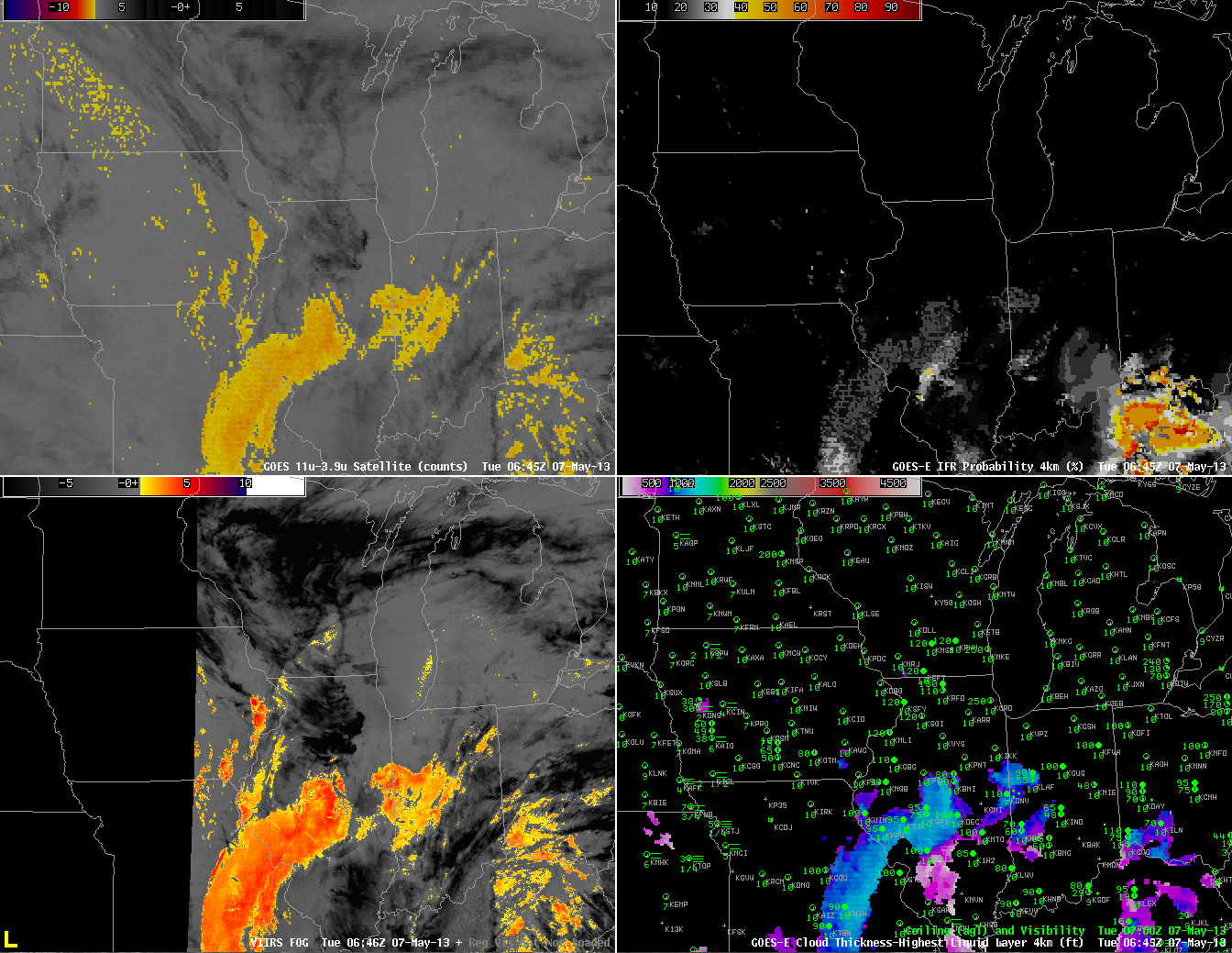
GOES-East Brightness Temperature Difference (10.7 µm – 3.9 µm) (Upper left), Suomi/NPP VIIRS Brightness Temperature Difference (10.35 µm – 3.74 µm) (Lower Left), GOES-R IFR Probability computed from GOES-East (Upper Right), GOES-R Cloud Thickness of highest water cloud (Lower Right), all imagery near 0645 UTC May 7 2013.

Areas of low stratus and fog developed over the upper Midwest in the morning on Tuesday, May 7th 2013.  In the image above from ~0645 UTC, both GOES and Suomi/NPP detect clouds comprised of water droplets over central Illinois southwestward through St. Louis and into central Missouri.  Careful examination of the ceilings/visibilities in that region, however, suggests that this is a mid-level stratus deck, and IFR Probabilities are suitably low.  Fog is observed in northwest Missouri and over western Iowa.  In this region, GOES does not detect water-based clouds, and IFR probabilities are low.

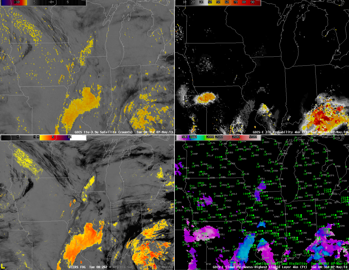
As above, but for times near 0830 UTC 7 May 2013

Two hours later, at 0830 UTC, (above) the mid-level clouds persist near St. Louis.  IFR conditions are not occurring there, however, and IFR probabilities are low.  IFR probabilities have increased around Kansas City, however, and they’re increasing in western Iowa as well, where numerous reports of reduced visibilities due to fog are occurring. This is a region where the brightness temperature difference product, the heritage method for detecting fog and low stratus, gives no information because of multiple cloud layers.

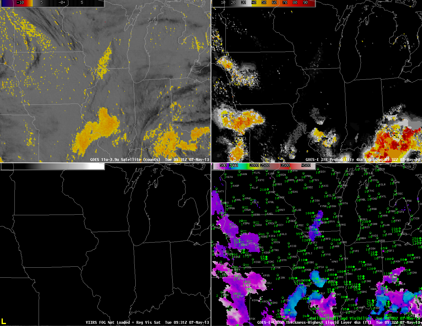
As above, but for times near 0930 UTC

At 0930 UTC (above), IFR Probabilities continue to increase over western Iowa southward into eastern Kansas, and they continue to be (correctly) suppressed near St. Louis where the traditional brightness temperature difference field notes the presence of a cloud comprised of water droplets.

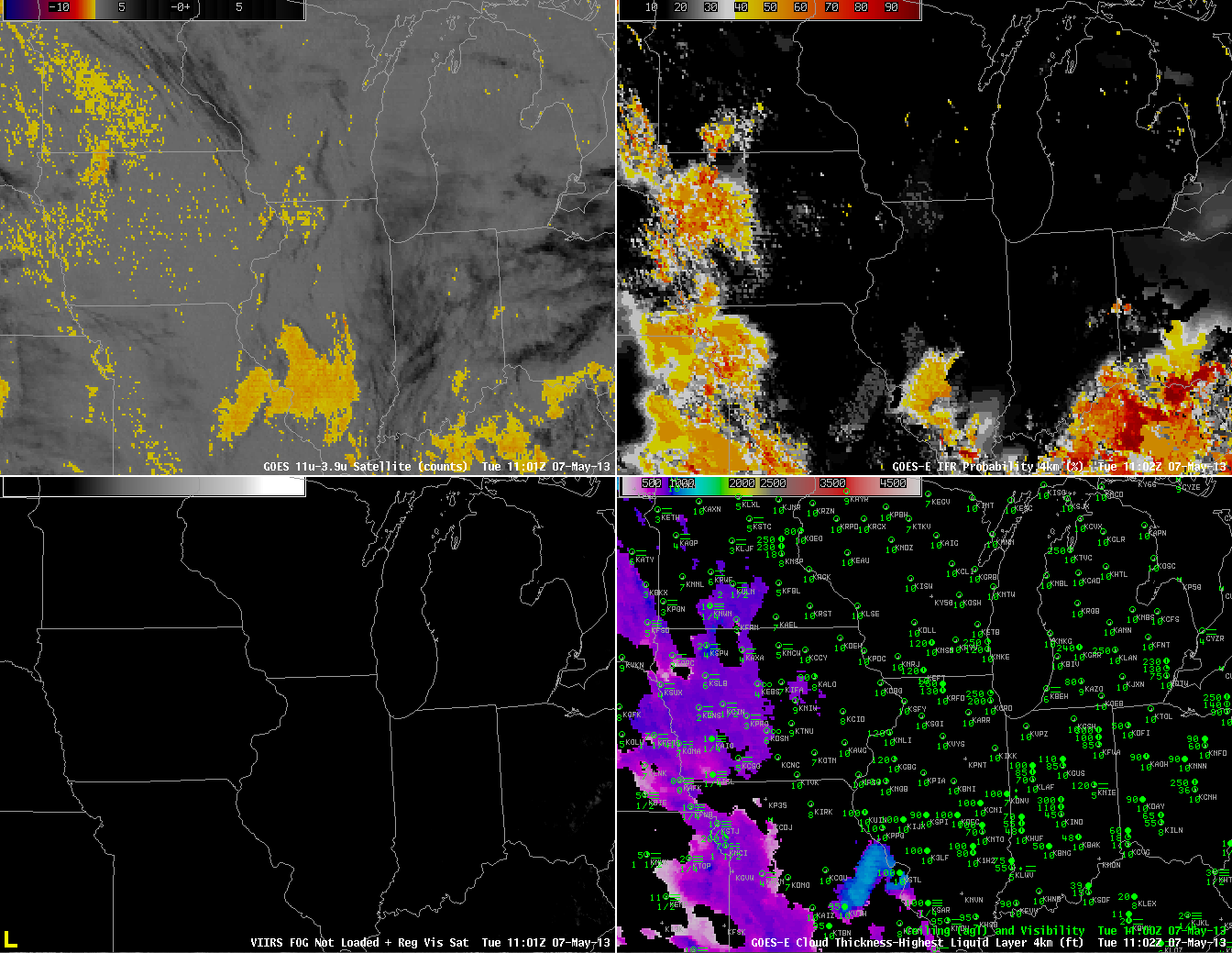
As above, but for 1100 UTC

By 1100 UTC (above), IFR probabilities are fairly high over most of western Iowa, western Missouri and eastern Kansas where many stations are reporting lowered ceilings and reduced visibility.  Again, this is a region where the traditional brightness temperature difference does not indicate the presence of fog and stratus.

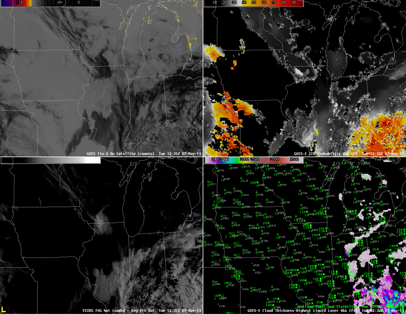
As above, but for 1230 UTC 7 May.  GOES-East Visible Imagery substituted for Suomi/NPP VIIRS Brightness Difference (bottom left)

 Shortly after sunrise, at 1230 UTC, above, IFR probabilities continue to be fairly high over western Missouri and eastern Kansas, a region where some stations are reporting IFR conditions (most notably in the Missouri River valley).  One reason that IFR Probabilities have dropped quickly over Iowa is that visible imagery shows no fog there, so the cloud-clearing part of the IFR Probability algorithm used during daytime conditions is operating properly.  Note also the false brightness temperature difference signal along the western shores of the Great Lakes.  This signal arises from a co-registration error between the longwave and shortwave infrared channels.  It continues through 1400 UTC (below).

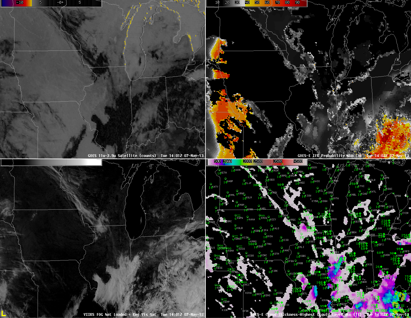
As above, but for 1402 UTC

Stratus over Southern California

VIIRS Day/Night Band (from Suomi/NPP), GOES-R IFR Probabilities (From GOES-West) and ceilings/visibilities, all near 0900 UTC on 30 April 2013

Day/Night imagery produced from VIIRS data on Suomi/NPP easily shows the large extent of marine stratus off the west coast of southern California at 0900 UTC on 30 April 2013.  That stratus may or may not be associated with low ceilings and reduced visibility that accompany IFR conditions.  A fused product that incorporates surface-based data will show where IFR conditions are most likely, and that is shown above as well.  Data from GOES-West and Rapid Refresh model output are combined to predict where IFR conditions are most likely.  Plotted observations of ceilings and visibilities confirm that the highest probabilities neatly overlay observed IFR conditions.  It is important to note that not all of the region covered by the marine stratus observed by the Day/Night band has IFR conditions.

The careful viewer may have noted that the IFR Probability fields over the ocean are quite high in regions where the Day/Night band shows no clouds at 0900 UTC.  GOES-R IFR Probabilities can be artificially enhanced in regions of Stray Light contamination in the GOES-West imager 3.7 data.  This contamination occurs around 0900 UTC at this time of year.   Note that by 1045 UTC (below), the stray light contamination has passed, and IFR probablilities over the ocean more properly align with the Day/Night band-observed cloud edges.

As above, but for 1045 UTC 30 April 2013

A similar set of imagery from 1045 UTC shows a general reduction in the predicted area of IFR probabilities, although the region of highest IFR probabilities, along the coast, persists and as do IFR conditions.

There was also fog over Monterey Bay on this morning.  Click here to read about it.

Radiation Fog over the Allegheny Mountains of Pennsylvania

GOES-R IFR Probabilities computed using GOES-East data, hourly from 0400 UTC through 1000 UTC (excluding 0500 UTC), 26 April 2013

GOES-R IFR Probabilities show a region over the Allegheny Mountains of northwest Pennsylvania slowly acquiring higher and higher probabilities, as ceilings and visibilities drop.  How did this product perform relative to traditional fog detection imagery (the brightness temperature difference product) and relative to data from Polar Orbiting satellites?  (The 0500 UTC imagery is excluded from the animation above because Stray Light Contamination in the 3.9 channel was apparent in the IFR probability fields).

GOES-R IFR Probability computed from GOES-East, 0332 UTC (Upper Left), GOES-East Brightness temperature Difference field (10.7µm – 3.9µm) at 0340 UTC (Upper Right), GOES-R Cloud Thickness (Lower left), GOES-R IFR Probability computed from MODIS data, 0328 UTC (Lower Left).

The ‘traditional’ method of fog detection that exploits emissivity difference of water clouds at 10.7µm and 3.9 µm, upper right in the figure above, at about 0330 UTC, just as the radiation fog was starting to develop, shows clouds detected over north-central Pennsylvania, but also from Centre County southwestward to the Laurel Highlands and to West Virginia.  GOES-based and MODIS-based IFR Probability fields have very low probabilities with these primarily mid-level clouds.

As above, but at 0615 UTC 26 April 2013

By 0615 UTC, IFR probabilities continue to increase over north-central Pennsylvania, and they remain low over southern and central Pennsylvania where mid-level clouds are reported (4100-foot ceilings at Johnstown, for example).

As above, but at 0740 UTC 26 April 2013

Another MODIS overpass at 0740 UTC better resolves the character of the developing fog and low stratus over north-central Pennsylvania.  Very high IFR probabilities in the MODIS-based fields outline the river valleys of the Allegheny Plateau in north-Central Pennsylvania.  GOES-based IFR Probabilities are high, but GOES lacks the resolution to view clearly the individual river valleys.

As above, but with Suomi/NPP brightness temperature difference (10.8 µm- 3.74µm) and Day-Night Visible imagery in the bottom right (0652 UTC), with the GOES-R IFR Probabilities (Upper Left), GOES-E Brightness Temperature Difference field (Upper Right), and GOES-R Cloud Thickness toggling between 0645 and 0702 UTC.

Suomi/NPP can also give information at high resolution about the evolving fog field.  The tendrils of fog developing in the river valleys are evident in the visible imagery created using reflected lunar illumination (A mostly full moon was present the morning of 26 April) and those water-based clouds are also highlighted in the Suomi/NPP Brightness Temperature Difference Field.  The clouds over the Laurel Highlands are higher clouds — they are casting shadows visible in the Day/Night band.

As in the figure above, but for 1015 UTC 26 April 2013

The final GOES-R Cloud Thickness field before twilight conditions, above, shows maximum thicknesses of 900 feet over Warren County, Pennsylvania, and around 850 feet over southern Clarion County.  According to this link, such a radiation fog will burn off in less than 3 hours after sunrise.  The animation below of visible imagery at 1315 and 1402 UTC shows the fog, initially widespread in river valleys at 1315 UTC mostly gone by 1402 UTC.

GOES-13 Visible Imagery, 1315 and 1402 UTC, 26 April 2013.  Warren and Clarion Counties are highlighted.

Fog over coastal North Carolina

GOES-R IFR Probabilities computed from GOES-East data, hourly from 0100 through 1200 UTC, 23 April 2013

A coastal storm along the east coast was responsible for low-level moisture over eastern North Carolina that resulted in IFR conditions.  Multiple cloud layers in the beginning of the animation above mean that IFR probabilities were computed using model data.  By 0315 UTC, however, upper level clouds had moved off the coast, leaving behind clouds at low layers that meant cloud data (brightness temperature difference) could influence the IFR probability fields;  consequently, the probability increased.  High clouds remained offshore, however, and the character of the IFR probability field shows the characteristic pixelated appearance over land — where satellite data are used in the computation of IFR probabilities — and the characteristic smoothed appearance over water where only model data are used to produce IFR probabilities.  Note how the highest IFR probabilities over eastern North Carolina do overlap the stations reporting IFR and near-IFR conditions.

GOES-R IFR Probabilities (Upper Left) computed using GOES-East, GOES-East Brightness Temperature Difference (10.7 µm- 3.9µm) (Upper Right), GOES-R IFR Probabilities computed using MODIS data (Lower Left).  All for times around 0715 UTC 23 April

The image above compares GOES-R IFR probabilities computed with MODIS and with GOES-East.  They do show very similar overall structures, with highest probabilities over land where the Brightness Temperature Difference field can contribute to the probability, and lower, smoother probability fields over water where only model data are used.  Note that both GOES-R IFR fields correctly ignore the low cloud signal over eastern South Carolina and central North Carolina.

GOES-R IFR Probabilities (Upper Left) computed using GOES-East, GOES-East Brightness Temperature Difference (10.7µm – 3.9µm) (Upper Right), Suomi/NPP Day/Night band from VIIRS (Lower Right).  Toggle for times 0615 and 0745 UTC 23 April

The GOES-based IFR probability field can also be compared to the Day/Night band sensed by VIIRS on board Suomi/NPP.  The 0609 UTC Day/Night band shows the effects of a near-full moon on the product.  The extensive cloud shield east of the Appalachians is visible, even though the image is at night, because of strong lunar illumination.  As with the traditional brightness temperature difference field, however, the cloud information from the Day/Night band gives little information about the cloud bases;  for that, the IFR probability field is needed, and low cloud bases are correctly restricted to extreme eastern North Carolina.  The Day/Night band at 0747 UTC is from a time after the moon has set;  only city lights and airglow are illuminating the clouds over Virginia and the Carolinas.  Cloud edges are still easily discerned.

Stratus and Fog over Texas

GOES-R IFR Probabilities (Upper Left) computed with GOES-East data, GOES-East Brightness Temperature Difference (10.7µm – 3.9µm) (Upper Right), Toggle between MODIS-based IFR Probabilities and Suomi-NPP Day-Night band imagery (Lower Left), Suomi-NPP Brightness Temperature Difference (Bottom Right) (10.8 µm- 3.74µm), all imagery around 0800 UTC

Stratiform clouds developed overnight in return flow from the Gulf of Mexico.  Some of the stratus was elevated, and some was closer to the surface creating IFR conditions.  The GOES imagery above captures the area of low clouds that are also visible in the Day/Night band — but the MODIS IFR Probability field suggests a difference in the stratus field near San Antonio.  Probabilities are far higher north of San Antonio’s latitude than south.  Surface observations suggest that IFR conditions are more likely where the MODIS-based IFR probabilities are highest.  (This demarcation line in the IFR Probability is far more noticeable in MODIS than in GOES).

Note that the GOES Brightness Temperature Difference field has a positive signal that is near the north-south oriented lakes in eastern Texas and western Louisiana, and that signal is absent from the VIIRS Brightness Temperature Difference field.  There is a misalignment between the 3.9 and 10.7 µm channels on GOES-13 (as discussed here) that has a maximum near 0900 UTC and that results in a false signal of low clouds.  This co-registration error can propagate into the IFR Probability field in regions where the Rapid Refresh is suggesting near-saturation at lower levels.

GOES-R IFR Probabilities (Upper Left) and surface observations of ceilings and visibility, GOES-East Brightness Temperature Difference (10.7  – 3.9) (Upper Right), Brightness Temperature at 10.7 (Lower Left) and 3.9 (Lower Right) at 1000 UTC (top image), 1215 UTC (middle image) and 1402 UTC (bottom image).

The demarcation between regions with IFR conditions and MVFR/VFR conditions becomes more distinct in the GOES-based IFR probability fields at 1000, 1200 and 1400 UTC, as shown above.  At all three times, the IFR probability field more accurately portrays the region of clouds that is most likely affecting aviation by displaying IFR conditions.

Fog/Low Stratus over San Francisco Bay

GOES-R IFR Probabilities computed from GOES-West, hourly from 0800 through 1500 UTC on 29 March 2013

The animation above shows the evolution of fog/low stratus as it moves inland from the Pacific Ocean into San Francisco Bay, and surroundings, on March 29th.  A chief forecast difficulty would be:  Will low ceilings impact San Francisco International Airport?  The TAF issued at 1212 UTC mentioned IFR conditions:

Fog Detection over Snow

GOES-R IFR Probabilities computed from GOES-East (Upper Left), GOES Brightness Temperature Difference (10.7 µm- 3.9 µm ) (Upper Right), Suomi/NPP 1.61 µm Reflectivity (Lower Left), Suomi/NPP Visible Imagery (0.64 µm) (Lower Right)

Snow cover in Spring promotes the development of advection fogs when relatively moist air moves over the snowpack and is cooled to its dewpoint, saturating.  But snowcover is also white when viewed from Satellite, and its presence makes the detection of fog areas difficult.  There are several products that can be used to distinguish between white snow and white clouds, and products that can be used to refine further the difference between stratus decks and fogbanks.

In the imagery above, Suomi/NPP 1-km resolution visible (0.64 µm) data in the bottom right figure show a large region of both clouds and snow over the North Dakota and surrounding US States and Canadian Provinces.  It is very difficult to find the cloud edges that are there.  The 1.61 µm imagery from Suomi/NPP is very helpful in screening out imagery of snow on the ground.  Water clouds are far more effective at reflecting radiation at wavelengths around 1.61 µm than snow or ice (snow and ice both strongly absorb radiation at that wavelength).  Thus, in the bottom left figure, the 1.61 µm reflectivity detected by Suomi/NPP, areas of snow appear dark and areas of water-based clouds are white.  This tells you where water clouds exist, but nothing about how high above the surface those water clouds are.  The brightness temperature difference product from GOES (10.7 µm – 3.9 µm) also highlights in dark regions of water-based clouds, but as with the 1.61 µm reflectivity does not give information about cloud bases.

The GOES-R Fog/Low Stratus IFR Probability neatly distinguished between the stratus deck over western Minnesota (that is not accompanied by IFR conditions at the surface) from the cloudy region over central and northern North Dakota that is accompanied by IFR conditions at the surface, as shown in the plotted observations.  (Thanks to Chad Gravelle for noticing this case today!)

One difficulty in Fog Detection

Toggle between Suomi/NPP Day/Night Band (i.e., Night-Time Visible Imagery, 0.70 µm) and Brightness Temperature Difference field (10.8 µm- 3.74 µm) at 0734 UTC on 28 March 2013

The image toggle above shows an area of stratus over central Missouri and surrounding states.  The stratus shows up in both the Night-time visible Day/Night band from Suomi/NPP (March 28th is one day past the Full Moon, so there is plenty of lunar illumination, and indeed lunar shadows from the higher cirrus clouds over Illinois, Kentucky and Tennessee are apparent).  The brightness temperature difference field crisply highlights the region of lower, water-based clouds.  That difference field arises from the differences in emissivity properties of the water-based clouds:  they emit nearly as a blackbody around 11 µm, and not as a blackbody at 3.9 µm.

A key question for this scene is:  is this cloud that is depicted stratus at mid-levels, or is it fog?  From the top (that is, as the satellite views it), a stratus deck will look very much like a fog bank.  The satellite gives little information, however, on how thick the cloud is, or on how close to the ground it sits.  A satellite-only fog detection algorithm, therefore, will include many false positives.

MODIS-based IFR probabilities, 0811 UTC on 28 March 2013

IFR probabilities include data about the surface that are incorporated into the Rapid Refresh Model.   This fused product clarifies where the brightness temperature difference product is detecting mid-level stratus versus low-level fog.  In this case over Missouri, IFR probabilities are very low throughout the scene because saturation at low levels in the Rapid Refresh is not occurring, and therefore IFR probabilities are low.

By blending information about the top of the cloud (the brightness temperature difference product) with information about the bottom of the cloud (the Rapid Refresh model data), a more accurate depiction of the horizontal extent of IFR conditions is achieved.