Category Archives: Pacific Northwest

Fog/Low Clouds over the Northwestern US

GOESBTD_IFR_20130909_1100

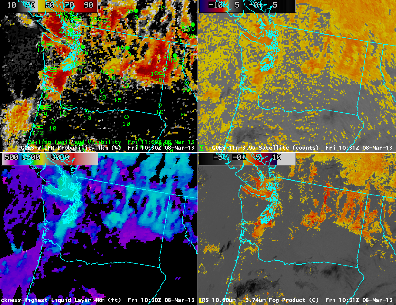
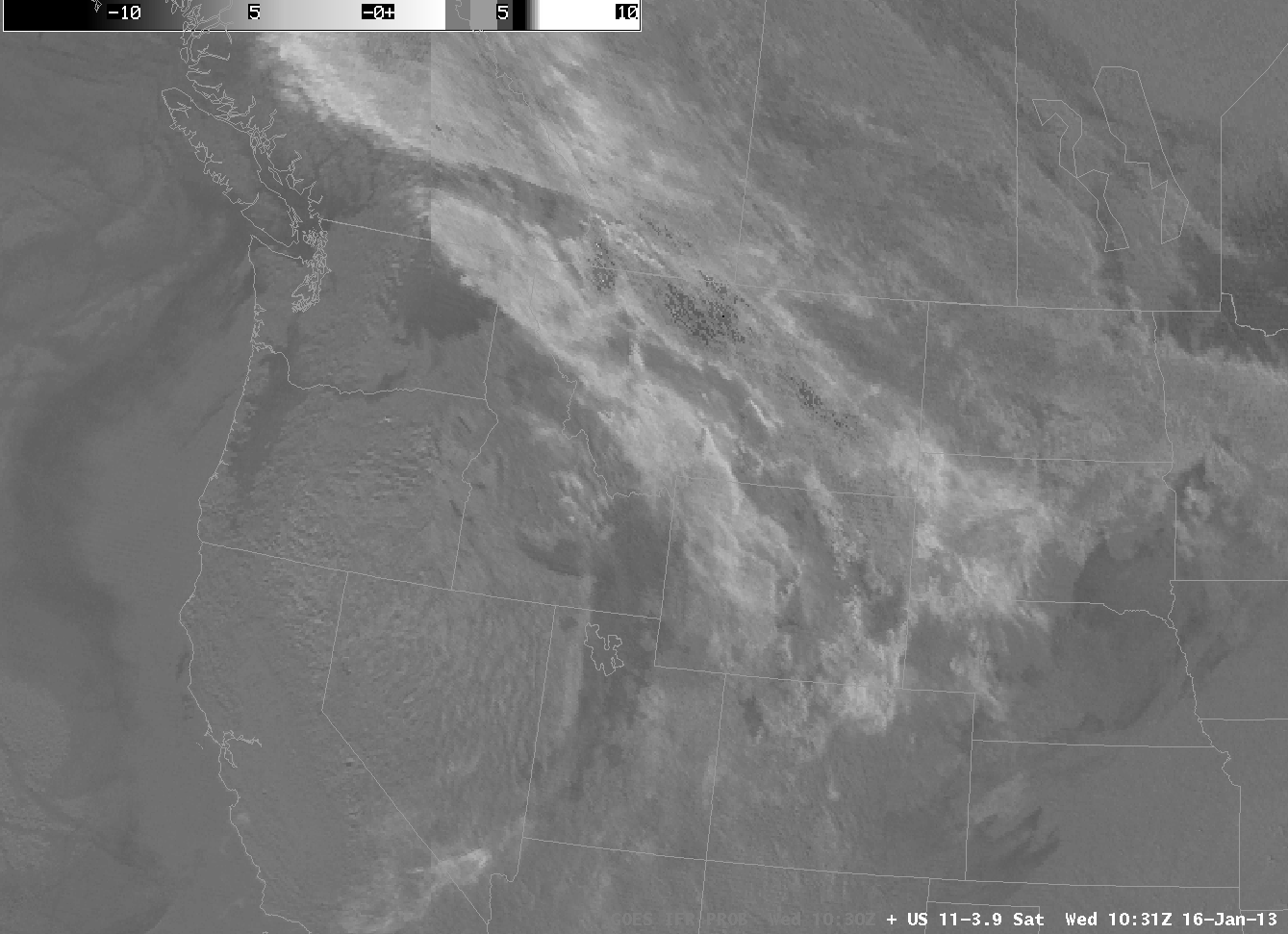
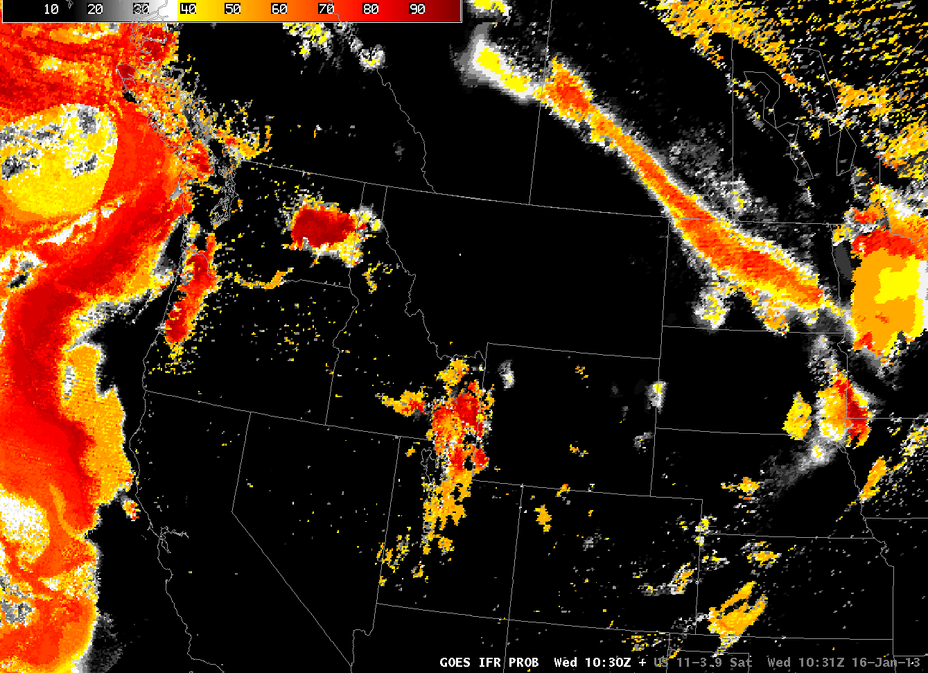
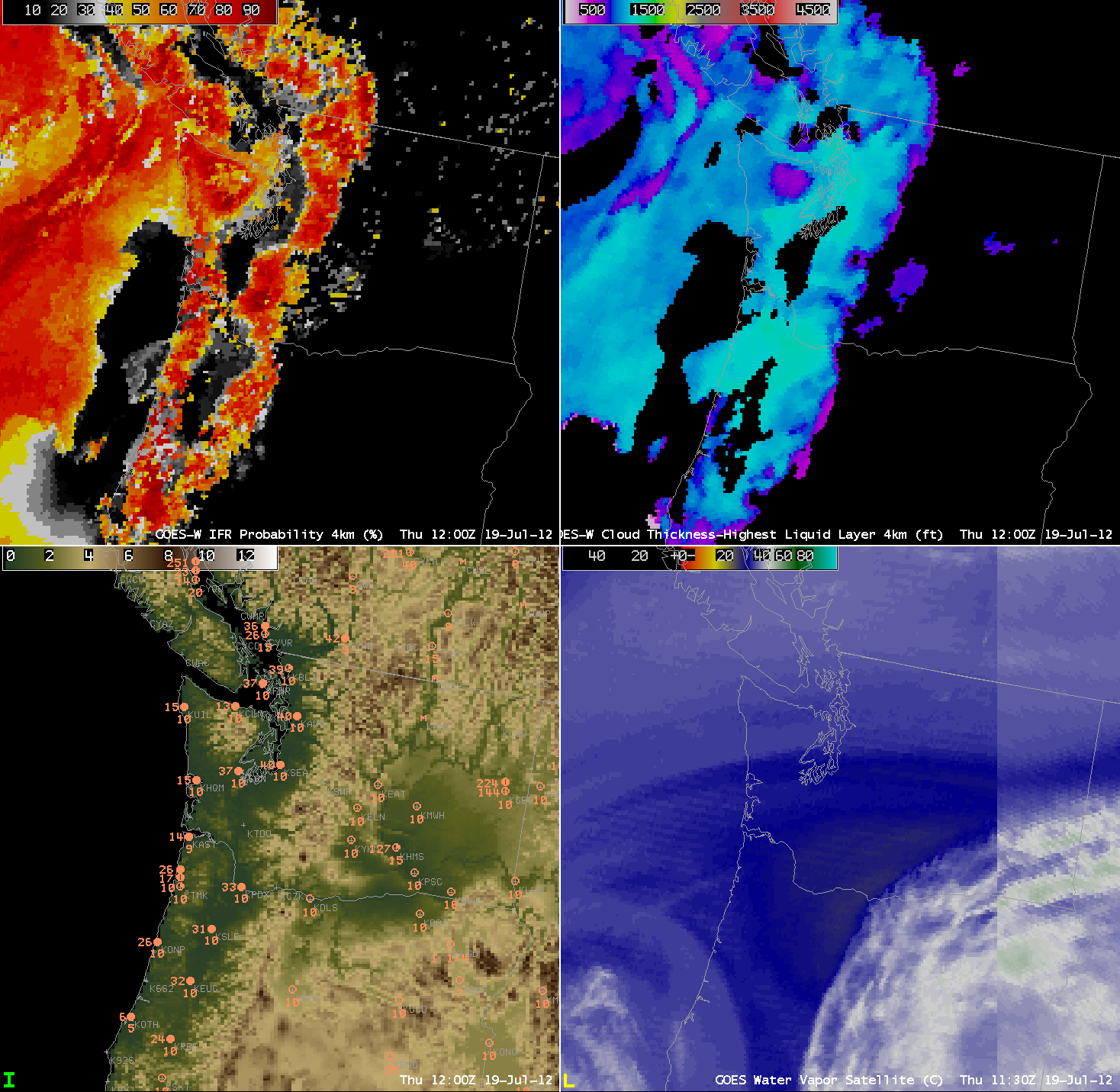
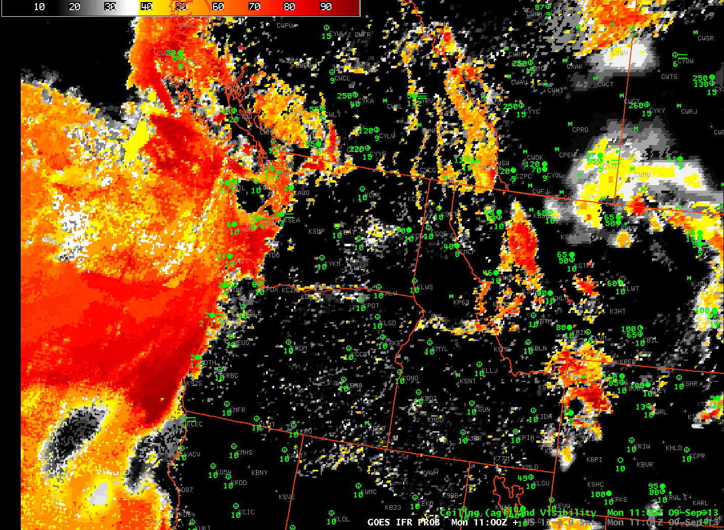
Brightness Temperature Difference from GOES-W and GOES-R IFR Probability computed from GOES-West and Rapid Refresh data, both images at 1100 UTC 9 September (click image to enlarge)

Fog and low clouds off the coast of Washington and in Montana are instructive in describing some strengths of the GOES-R IFR Probability algorithm. A general statement is that the IFR Probability improves — sometimes greatly — the approximation of where fog and low clouds are present. In the example above, the brightness temperature difference shows a positive signal — suggestive of low clouds — along the Washington and Oregon coasts (where IFR conditions are reported within the marine layer of stratus/fog). The brightness temperature difference also has a strong signal over Montana; there is a scattershot signal as well over Nevada, Idaho and western Oregon/Washington. These are regions where the GOES-R IFR Probability field is correctly minimizing the probability of fog/low clouds. Over Montana, the Brightness Temperature Difference signal is driven by an elevated stratus deck. The positive signal in arid Nevada, Idaho, Oregon and Washington arises from soil emissivity variability. The IFR Probability field maintains a strong signal where IFR conditions are reported, and reduces the strong signal in regions where fog/low stratus likely do not exist.

BTD_GOES_VIIRS_20130909_1100

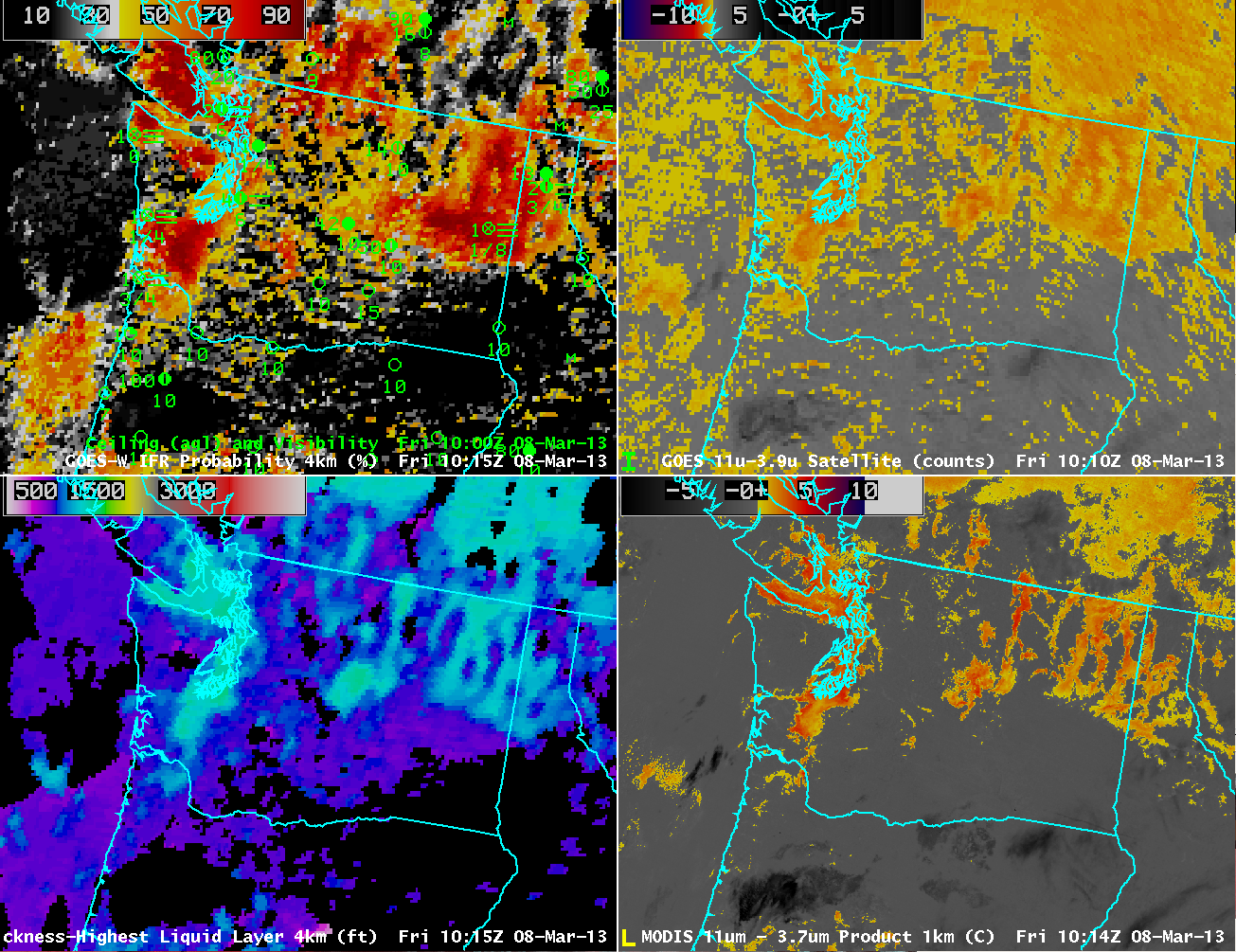
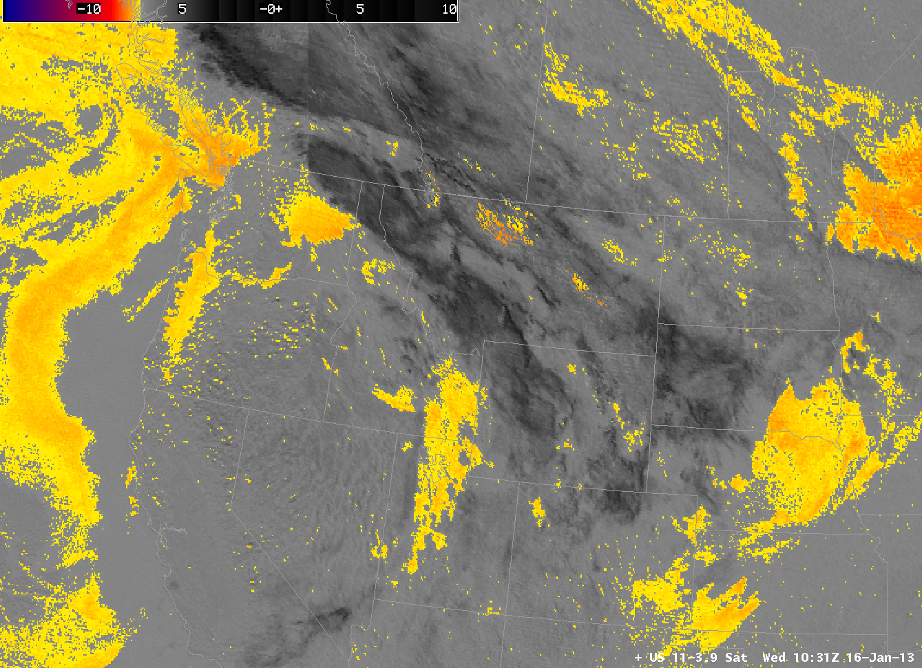
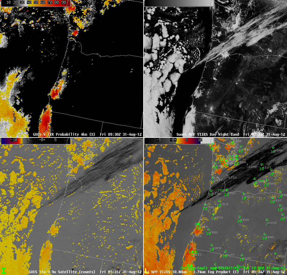
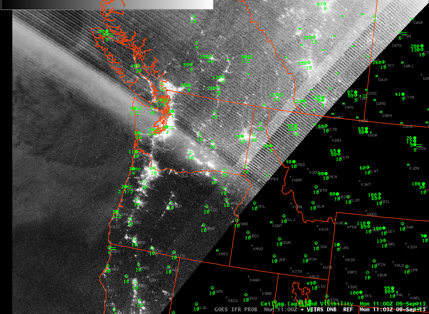
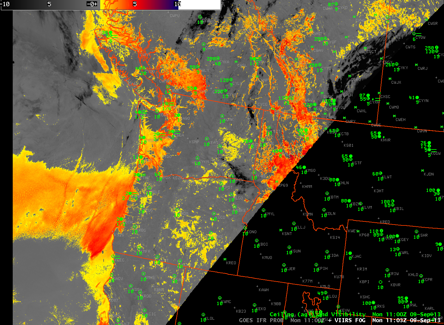
Brightness Temperature Difference from GOES-W and and from Suomi/NPP, both images at ~1100 UTC 9 September (click image to enlarge)

Suomi/NPP was passing over the Pacific NW at 1100 UTC, the times of the imagery above, and it provided a higher-resolution look. Suomi/NPP data allows for better definition of the — apparently — thickest stratus/fog layer right along the Washington and Oregon coast. The superior resolution also allows for a better approximate of the dendritic nature of river valley clouds, as demonstrated over southern British Columbia. However, the brightness temperature difference here is also unable to distinguish between fog on the ground and stratus that at mid levels.

PacNW_FOG_20130909_1100

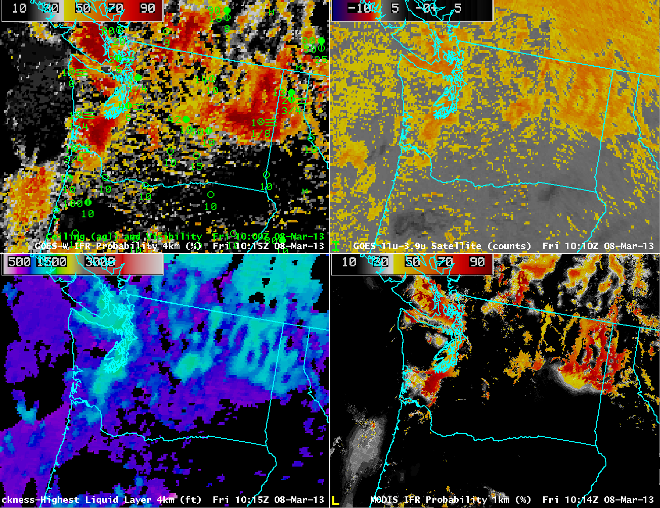
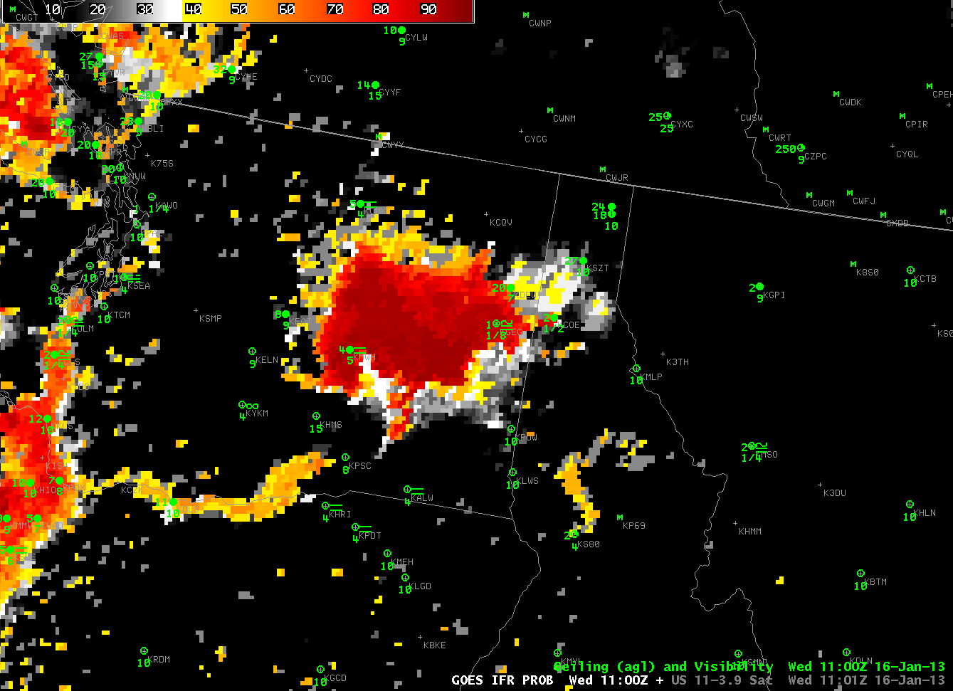
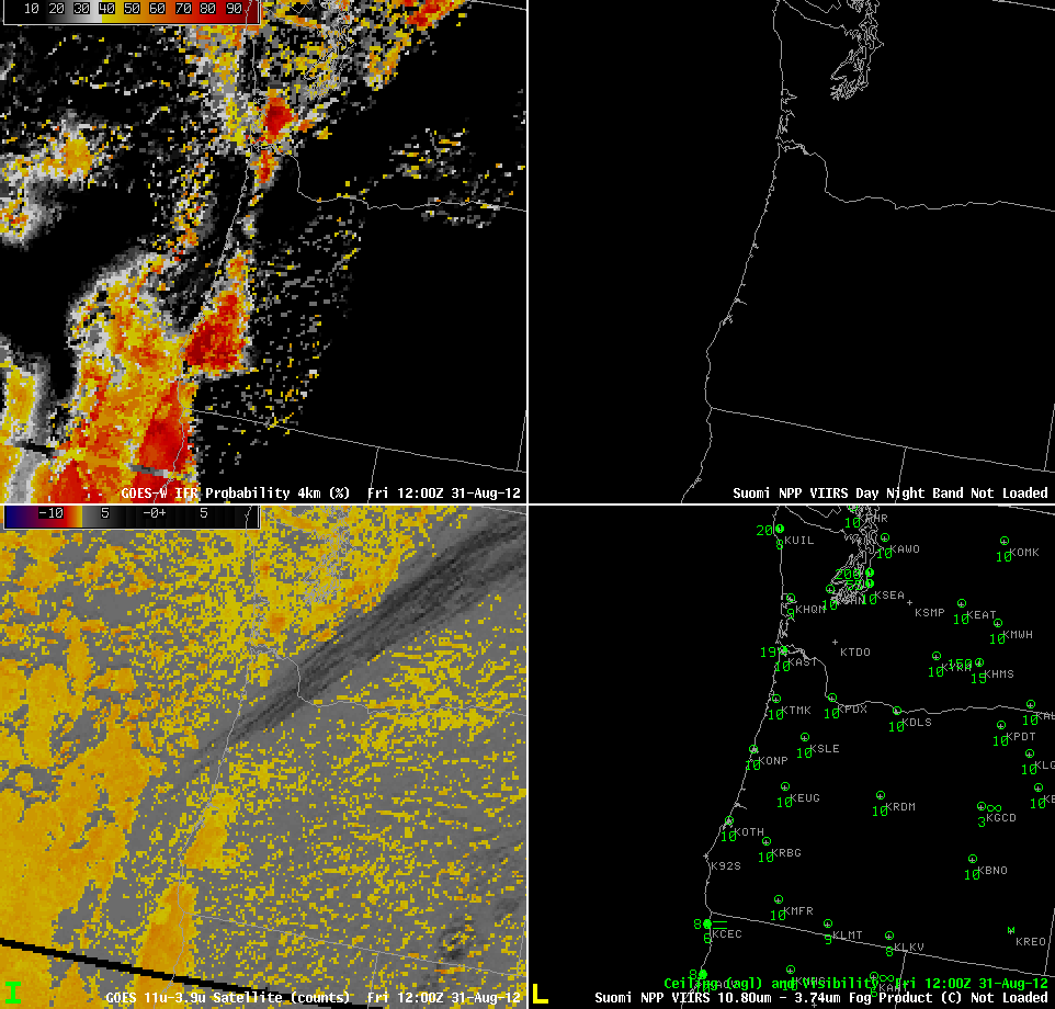
Brightness Temperature Difference from GOES-W, Day/Night Band, Brightness Temperature Difference from Suomi/NPP, Day/Night Band, GOES-based GOES-R IFR Probabilities, all at ~1100 UTC 9 September (click image to enlarge)

The animation above loops through the GOES-Based Brightness temperature difference, the Suomi-NPP Brightness temperature difference, the Suomi-NPP Day/Night band, and the GOES-R IFR Probability field computed with GOES-W and Rapid Refresh data.

Low clouds in the Pacific Northwest

GOES-R IFR Probabilities computed from GOES-West (Upper Left), GOES-West Brightness Temperature Difference (10.7 µm – 3.9 µm) (Upper Right), GOES-R Cloud Thickness from GOES-West (Lower Left), GOES-R IFR Probabilities computed from MODIS (Lower Right), hourly from 0500 through 1200 UTC on 23 July 2013.

Hourly GOES-R IFR Probabilities ably capture the creep of low fog and stratus into Puget sound from the north — through the strait of Juan de Fuca, and from the south, with low clouds eventually surrounding the Olympic Mountains.  Part of the input into the GOES-R IFR Probability algorithm is the brighness temperature difference shown in the upper right, and note that it used alone overpredicts where low clouds/fog might be occurring.  Including Rapid Refresh data allows the GOES-R algorithm to restrict — correctly — the IFR conditions to where they are most widespread.

Suomi-NPP data from the VIIRS instrument includes a Day/Night band that on July 23rd, when the moon was approaching full, neatly outlines both the cloudy regions — where moonlight is reflected off clouds — and those regions where light is being emitted (that is, cities).

As above, but with the VIIRS Day/Night band in the bottom right, at 0923 and 1103 UTC.

Suomi/NPP VIIRS data also includes 10.8 and 3.74 µm imagery, so a brightness temperature difference product can be computed (work is in progress to incorporate Suomi/NPP data into the GOES-R algorithm suite so an NPP-based IFR probability can be developed.  The toggle below compares the day/night band data with the brightness temperature difference produce at 0923 UTC.

Fog Detection on Oregon’s West Coast

Toggle between MODIS-based and GOES-West-based IFR Probabilities, ~0630 UTC 01 July 2013

The high-resolution MODIS data likely gives a more accurate interpretation of visibility obstructions near the surface because it better resolves the sharp edges to fog/low stratus that can occur along the west coast of the United States, as exemplified by this scene centered on Oregon.  Look at North Bend, OR, for example.  In a hole in the MODIS field, but with relatively high probability in the GOES field.  The MODIS field also highlights ship fields in the stratus deck off the coast.

MODIS data is useful for high spatial resolution, but the temporal resolution at one point is not good.  The swath width on Suomi-NPP is wide enough, however, that sometimes two sequential polar passes will overlap over the northern United States, giving a 90-minute time-step with high-resolution data.

Brightness Temperature Difference, 11 – 3.74 from VIIRS data on Suomi/NPP.

The animation above shows how the low clouds, as detected using the Brightness Temperature Difference between 3.74 and 11 channels from VIIRS, are moving inland btween 0935 and 1116 UTC on 1 July.  The brightness temperature difference also shows a general increase offshore, so the likelihood of any breaks in the low clouds is decreasing.  The Day/Night band imagery shows a similar change in low clouds along the coast, although the view is somewhat obscured because this region is in the stray light zone (that is, the satellite is illuminated by the sun even though it is over a region where it is still night).

Day/Night band imagery along the west coast, 0935 and 1116 UTC on 1 July
GOES-R IFR probabilities, 0930 and 1115 UTC, 1 July 2013

GOES-R Probabilities computed from the GOES-West imager also show an expansion in the region where IFR probabilities are highest.  Thus, the expansion in low clouds detected by the VIIRS instruments on Suomi/NPP likely corresponds an increase in the area with lowered visibilities.

Cold frontal passage in Oregon

GOES-R IFR Probabilities (Upper Left), GOES-West Brightness Temperature Difference (10.7 µm – 3.9 µm) (Upper Right), Topography (Lower Left), GOES-West Water Vapor Imagery (6.7 µm) (Lower Left), hourly from 0400 through 1700 UTC 20 March 2013.

The animation above of the Fog/Low Stratus and Brightness Temperature difference highlights the difficulty that the traditional brightness temperature difference product encounters when multiple cloud layers are present, as you might expect to be present given the water vapor imagery.  At the beginning of the animation, highest IFR probabilities exist over the elevated terrain that surrounds the Willamette Valley in Oregon.  There were also high probabilities off shore.  As the frontal region moves onshore, IFR probabilities increase on shore.   Note also how the GOES-R IFR Probability field is a more coherent one whereas the traditional brightness temperature difference field from GOES contains many separate areas of return that make it harder to see the big picture.  The brightness temperature difference also suffers from stray light contamination at 1000 UTC — but that contamination does not propagate into the GOES-R IFR probability field.

GOES-R IFR Probabilities computed from GOES-West (Upper Left), GOES-West Brightness Temperature Difference (10.7 µm – 3.9 µm) (Upper Right), Topography (Lower Left), Toggle between Suomi/NPP Brightness Temperature Difference (10.8 µm – 3.74 µm) and Day/Night Band, all imagery near 1000 UTC on 20 March 2013

The imagery above shows how straylight contamination in the shortwave IR (3.9 µm) can influence the brightness temperature difference.  The GOES imagery shows the effects (just at this 1000 UTC image, which is also included in the animation above), but that ‘contamination’ does not propagate strongly into the GOES-R IFR Probability.  Note also that the Suomi/NPP Brightness Temperature Difference shows none of the stray light contamination.  Lunar illumination  allows the nighttime visualization of the clouds off the west coast of the US.  As this frontal band moves over Oregon, reduced visibilities result, but only the GOES-R IFR probabilities accurately capture the location of the frontal band because of the multiple cloud layers that exist.

Resolution Issues over the Pacific Northwest

GOES-R IFR Probabilities computed from GOES-West (Upper Left), GOES-E/W Brightness Temperature Difference (10.7 µm – 3.9µm) (Upper Right), GOES-R Cloud Thickness (Lower Left), Suomi/NPP VIIRS Brightness Temperature Difference  (Lower Right)
As on top, but with MODIS Brightness Temperature Difference (11 µm – 3.7 µm) in the bottom right.

The imagery above underscores the power of higher resolution on fog detection.  The images on the right side of the images are brightness temperature difference fields, the heritage method for detecting fog and low stratus.  The GOES field (top right) actually includes data from GOES-East (eastern Washington and points east — a faint seam is discernible in the image) and GOES-West (western Washington).  Pixel size over Washington is large — 6 or 8 kilometers (vs. 4 kilometers at the subsatellite point).  In contrast, Suomi/NPP VIIRS data and MODIS data (bottom right) has a resolution of 1 km.  The brightness temperature difference from MODIS and VIIRS more easily resolves the fine-scale structure of the topographically influenced or topographically constrained fog and low stratus.  The brightness temperature difference field from GOES is one of the predictors used to generate the IFR Probabilities shown in the upper right.  When poor resolution smears out the horizontal domain of the fog and low stratus in the brightness temperature difference field, you might expect a similar effect on the IFR probabilities.

As above, but with MODIS-based GOES-R IFR Probabilities in the lower right

 MODIS data can be used to compute IFR probabilities.  Compare the lower right and upper left figures.  High MODIS IFR Probabilities are far more restricted to regions where IFR conditions are observed.  In contrast, GOES-based IFR probabilities seem to leak into regions where IFR conditions are not reported.

The higher resolution MODIS-based IFR Probabilities (and coming soon, Suomi/NPP-based IFR probabilities) nicely complement the higher temporal resolution of the GOES imagery.  Ideally, use of the changes in the GOES-based IFR probabilities shows how IFR conditions evolve over the course of a night.  These changes should be tempered with knowledge of the limitations of the horizontal resolution of GOES that are highlighted in the above imagery.

Fog/Low Stratus in eastern Washington State

Brightness Temperature Difference plot over the NW USA, 1031 UTC 16 January

The plot above shows the default enhancement the brightness temperature difference product traditionally used to highlight regions of low clouds and fog.  The greyscale nature of the product can make interpretation difficult.  However, if a suitable enhancement is applied (below), such that fog and low clouds are enhanced, interpretation is easier.

As above, but color-enhanced.

This image suggests the presence of fog or low stratus (or both) off the west coast of the US, in and around Salt Lake City, near Spokane, and in the Willamette Valley and Columbia River Valley.  It is difficult to tell if the regions are associated with restrictions in visibility because an elevated stratus deck and a fog bank look very similar in the brightness temperature difference field.  Therefore, the GOES-R Fog/Low Stratus IFR Probability field was developed to highlight regions where IFR conditions are most likely.  That product is shown below.

GOES-R IFR Probabilities, 1030 UTC on 16 January

Compare the IFR probability field to the Brightness Temperature Difference field above it.  Several things are apparent.  Highest probabilities for visibility restrictions are centered near Spokane, WA.  There is a region of higher IFR probabilities in North Dakota that is missing entirely in the Brightness Temperature Difference product.  IFR probabilities over Utah vary more than the Brightness Temperature Difference signal.  The differences all arise from the model data that are used to better highlight where low-level saturation is occurring.

IFR Probabilities and observations of Ceilings/visibilities from 1100 UTC on 16 January.

This zoomed-in imagery shows that, indeed, visibility restrictions (IFR conditions) are occurring in eastern Washington.  The strength of the fused product is that is provide a coherent signal over a larger area, so you can better define the region of IFR conditions than is possible with surface observations alone.  The region of higher IFR probabilities over North Dakota is also associated with IFR and near-IFR conditions in a northwest-southeast oriented strip including Harvey and Jamestown, ND (not shown).

GOES-R Fog and the Day/Night Band on VIIRS

GOES-R IFR Probabilities (upper left), Suomi/NPP VIIRS Day/Night Band (upper right), Brightness temperature difference (10.7 micrometers – 3.9 micrometers) from GOES (lower left), Brightness temrperature difference (11.35 micrometers – 3.74 micrometers) from Suomi/NPP VIIRS (lower right), all around 0930 UTC on 31 August.

The presence of the Day/Night band on the VIIRS instrument on the Suomi/NPP satellite offers a unique method of validating the presence of fog or stratus at night.  During times near full moon (such as the Blue Moon on 31 August), the Day/Night band can detect low clouds using light reflected from the moon.  The GOES-R IFR probabilities show fog and low/stratus over southwestern Oregon;  a larger region of fog/low stratus stretched from just north of Crescent City, CA (where IFR conditions are reported) southward down the coast.  Note also a small patch over southwestern Washington and coastal northwest Washington (where IFR conditions are reported.  Cirrus clouds that prevent the detection of fog/low stratus from satellite are present stretching northeastward from the ocean off the central Oregon coast into central Washington.  There is a small signal in the GOES-R IFR Probability field underneath this upper cloud feature.

GOES-R IFR probabilties (Upper left), Suomi/NPP VIIRS day/night band (upper right), GOES-West Brightness Temperature Difference between 10.7 and 3.9 micrometer channels (Lower left), Observations (Lower right), all around 1200 UTC, 31 August

AT 1200 UTC, some benefits of the GOES-R IFR probability field are apparent.  The noisy signal over central and eastern Oregon is reduced, and a signal is present also underneath the thin cirrus streak that persists over extreme northwest Oregon.

GOES-R IFR as a ‘cleaner’ Product

Image toggle between 0800 UTC GOES-R IFR Probability and GOES-West Brightness Temperature Difference between 10.7 and 3.9 micrometers

Because the GOES-R IFR Probabilty product uses multiple predictors in its computation of probabilities, regions where the satellite returns give erroneous signals — because of soil emissivity property changes, for example — can be suppressed if the Rapid Refresh strongly suggests fog is unlikely in that region.  In this example over the Pacific Northwest on the morning of 25 July, both products correctly suggest IFR conditions are likely along the coast (and observations are congruent with that suggestion).  The ‘traditional’ brightness temperature difference product, however, shows a signal over central and western Washington.  IFR conditions are not present there.  The GOES-R IFR product de-emphasizes the satellite signal there.  This ably demonstrates a benefit in using a fused product.

Terrain

GOES-R IFR Probabilities (Upper left), GOES-R Cloud Thickness (Upper right), Terrain with surface plots of Ceiling (above MSL) and visibility (lower left) and the GOES-15/GOES-13 Water vapor imagery

When terrain rises up into the clouds, IFR conditions occur, and the GOES-R IFR product shows that effect.  These images from ~1200 UTC on 19 July 2012 show two regions of IFR conditions over the Pacific Northwest — along the spine of the coastal range from the Olympic Mountains south to the Oregon Coast Range and along the Cascades from east of Seattle southward to Oregon.  The observations shown in the lower left (with ceilings above mean sea level, plotted over topography) are consistent with the IFR probabilities:  Low probability over the region between the coastal range and the Cascades, and high probability in regions over the Cascades where the height exceeds the observed ceilings over, say, Seattle and Portland, and high probabilities along the Coastal Range where heights exceed the observed ceilings along the coast.

Cirrus Effects in GOES-R Fog/Low Stratus Prediction

MODIS-based IFR Probabilities (Upper Left), Cloud Thickness of the Highest Liquid Layer (Upper Right), 3.7 micron brightness temperatures (Lower Left) and MODIS Cloud Phase (Lower Right) from 1100 UTC on 12 July 2012.

A benefit of the GOES-R Fog/Low Stratus product is that it provides a signal even in the presence of higher clouds that make fog detection via brightness temperature difference methods impossible.  In this case from 1100 UTC on 12 July, a thin cirrus shield off the coast of Oregon (the bright white wisp in the 3.7 micron imagery in the bottom left) shows up (correctly) as an ice cloud in the cloud phase field (bottom right).  Note that low cloud thickness is not computed when higher clouds overlay the low cloud field — so data are available underneath the cirrus deck, although you might infer the thickness from the surrounding fields.  The GOES-R IFR probabilities show values exceeding 50% underneath the cirrus deck, in a region where the brightness temperature difference gives no information.

This effect is also seen in GOES-based imagery, below, from 1200 UTC.  The Cirrus cloud has moved onshore just south of KONP (Newport, OR) where IFR conditions exist.  The IFR probabilities suggest fog/low clouds are likely present in a region where the brightness temperature difference field gives no information because of cirrus clouds.  Although this cirrus shield is small, it should be easy to envision a larger cirrus shield and what that impact might be.

Note also the number of false positives in the brightness temperature difference field that do not show up in the IFR Probabilities.

GOES-West-based Cloud Thickness of the Highest Liquid Layer (Upper Left), IFR Probabilities (Upper Right), 11 micrometer – 3.9 micrometer brightness temperature difference (Bottom Left) and Cloud Phase (Bottom right)