Category Archives: Multiple Cloud Layers

IFR Probabilities with an Early Spring storm system

GOES-R IFR Probabilities (Left) and Brightness Temperature Differences (Right) Computed from GOES-East (Top) and MODIS (Bottom)

The multiple cloud layers that are common with an extratropical cyclone preclude identification of fog/low clouds by traditional brightness temperature difference methods because low clouds are overlain by mid-level and higher clouds. Thus, the satellite is unable to view them.  In the images above from early morning on 11 April over the midwest, both GOES and MODIS detect low clouds over southern Iowa and Missouri.  The GOES-R IFR Probability fields show enhanced probabilities over a larger region that stretches from northern Ohio westward to southwestern Minnesota, and southward from Iowa to Missouri.  Observed ceilings show IFR (or near-IFR) conditions from northwest Ohio westward to northern Iowa.  Regions of model-based enhanced IFR probabilities capture this region of IFR conditions.  IFR ceilings also exist under the region where the traditional brightness temperature difference field has a strong signal.  When interpreting the IFR probability fields, it is important to recognize the differences that arise due to differences in the predictors used (for example, between the higher IFR probabilities over southeast Iowa — where satellite and model data are used — and the lower probabilities over north central Iowa where only model data are used).

Observed Ceilings, in feet, over the midwest, 0900 UTC on 11 April 2013

Fog/Low Stratus Examples on both Coasts

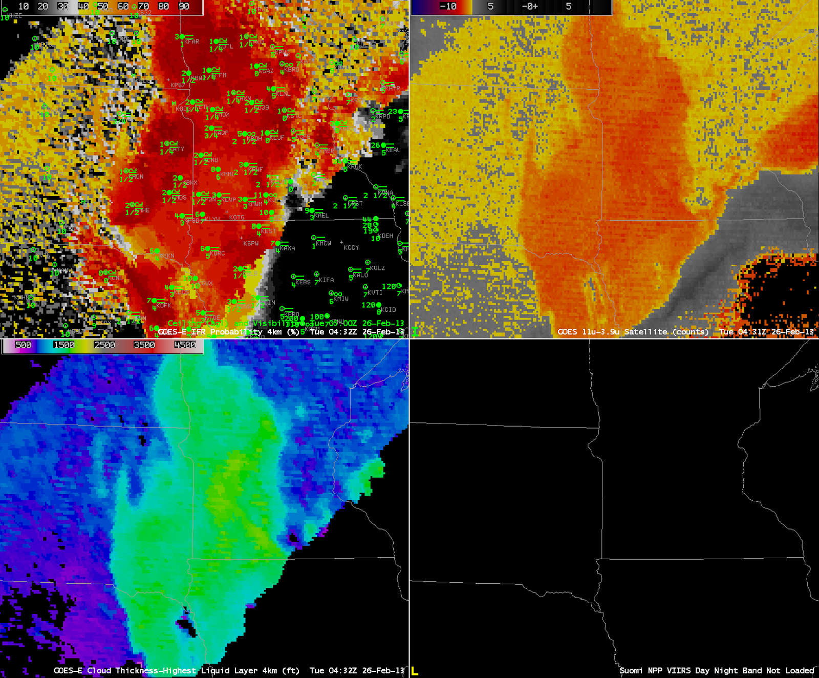
Two different systems — one approaching California, and one in the Gulf of Mexico — provide examples of how the GOES-R Fog/Low Stratus algorithm give information about visibilities and ceilings in regions where high clouds obscure the satellite view of low levels.

GOES-R IFR Probabilities computed from GOES-West, hourly, from 0700 through 1700 UTC 4 April 2013

The first case, off the West Coast, starts with a deck of high clouds over the coast associated with a landfalling cyclone.  IFR Probabilities over the Pacific near the California coast are initially derived solely from Rapid Refresh model data.  Consequently, IFR probabilities are not high.  As the cirrus shield pushes inland, low clouds become visible to the satellite, and when both satellite and model predictors are used to compute IFR Probabilities, higher probabilities are a result.  In addition, small-scale variability that is inherent in a satellite image (and perhaps not so inherent in model output) changes the character of the IFR Probability field from a flat field at the start to a more pixelated field later in the animation.  As the low clouds push onshore, associated moisture and precipitation helps to generate near-IFR and IFR conditions in regions where the IFR Probabilities are depicted to be high.

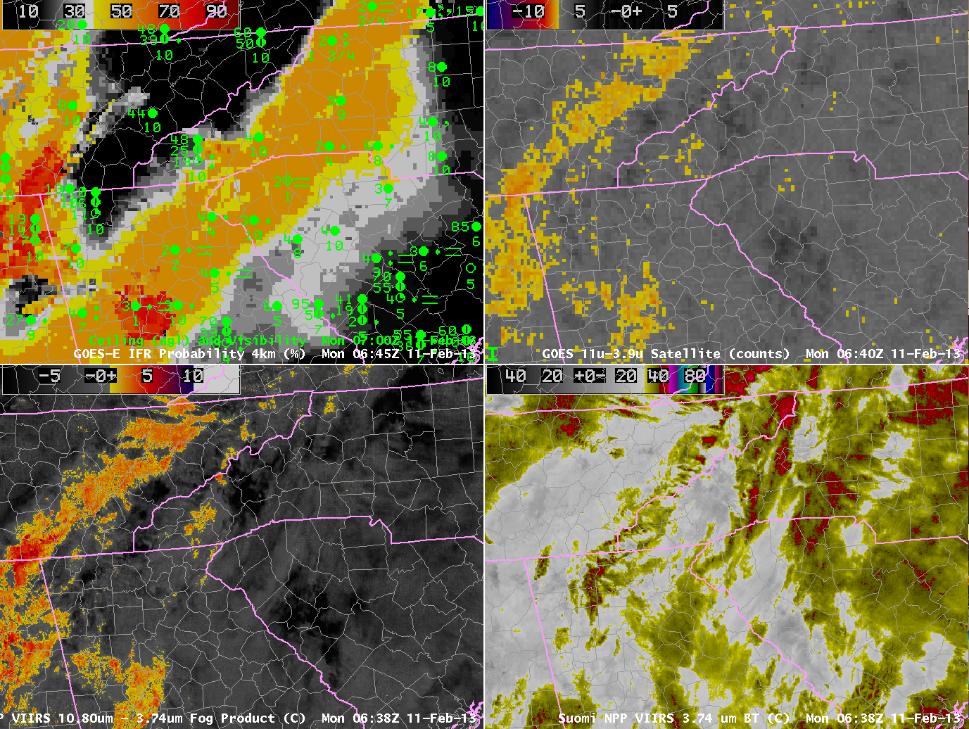
The second case, below, over the deep South, shows a region of fog/low clouds moving over Georgia as mostly model-based IFR Probabilities also move over the state.  Strong convection over the Gulf of Mexico produced abundant high-level cloudiness;  thus, IFR Probabilities could only be computed using Rapid Refresh Data over Georgia  — but the computed IFR Probabilities both outline the region of lowest ceilings/visibilities and match their slow spread to the north and east into South Carolina.  The IFR Probability field over Mississippi has a more pixelated look to it, and shows higher values, because satellite data are also used to diagnose the IFR Probability:  IFR Probabilities are highest only where both predictors (model and satellite) are used.

GOES-R IFR Probabilities computed from GOES-East, hourly, from 0702 UTC through 1745 UTC, 4 April 2013

IFR Probabilities during a Winter Storm

GOES-R IFR Probabilities computed from GOES-East and Rapid Refresh model output, from 0100 through 1400 UTC on March 25 2013

A late winter storm moving through the mid-Altantic states was responsible for an episode of reduced visibilities.  The loop above shows two areas of reduced visibilities initially — one over the Piedmont of Georgia, the Carolinas and Virginia, and one over the Ohio River Valley.  Visibilities decrease as the higher IFR probabilities move in, and, conversely, increase as the higher probabilities move out.  IFR Probabilities over southern Ohio, for example, have a character that suggests the probabilities have been computed chiefly with model data.  Probabilities are somewhat reduced, and the fields are not pixelated (as they are over the Carolina Piedmont, for example).

GOES-R IFR Probabilities computed from GOES-East, Brightness Temperature Difference fields from GOES-East (10.7 µm – 3.9 µm) and from Suomi/NPP (10.8 µm- 3.74 µm) around 0700 UTC on 25 March 2013

The animation of the ~0700 UTC IFR Probability and brightness temperature difference field from both GOES-East and from the polar-orbiting Suomi/NPP, above, shows another strength of the IFR Probability product:  It screens out regions where high stratus give a signal.  The top of a stratus deck and the top of a fog deck may have a very similar brightness temperature difference signal.  By fusing the satellite data with a product that includes surface information (such as output from the Rapid Refresh Model), regions with elevated stratus, which clouds do not significantly impact aviation operations, can be removed from the signal.  Only regions with actual surface observation restrictions are highlighted in the IFR probability signal above.

Cold frontal passage in Oregon

GOES-R IFR Probabilities (Upper Left), GOES-West Brightness Temperature Difference (10.7 µm – 3.9 µm) (Upper Right), Topography (Lower Left), GOES-West Water Vapor Imagery (6.7 µm) (Lower Left), hourly from 0400 through 1700 UTC 20 March 2013.

The animation above of the Fog/Low Stratus and Brightness Temperature difference highlights the difficulty that the traditional brightness temperature difference product encounters when multiple cloud layers are present, as you might expect to be present given the water vapor imagery.  At the beginning of the animation, highest IFR probabilities exist over the elevated terrain that surrounds the Willamette Valley in Oregon.  There were also high probabilities off shore.  As the frontal region moves onshore, IFR probabilities increase on shore.   Note also how the GOES-R IFR Probability field is a more coherent one whereas the traditional brightness temperature difference field from GOES contains many separate areas of return that make it harder to see the big picture.  The brightness temperature difference also suffers from stray light contamination at 1000 UTC — but that contamination does not propagate into the GOES-R IFR probability field.

GOES-R IFR Probabilities computed from GOES-West (Upper Left), GOES-West Brightness Temperature Difference (10.7 µm – 3.9 µm) (Upper Right), Topography (Lower Left), Toggle between Suomi/NPP Brightness Temperature Difference (10.8 µm – 3.74 µm) and Day/Night Band, all imagery near 1000 UTC on 20 March 2013

The imagery above shows how straylight contamination in the shortwave IR (3.9 µm) can influence the brightness temperature difference.  The GOES imagery shows the effects (just at this 1000 UTC image, which is also included in the animation above), but that ‘contamination’ does not propagate strongly into the GOES-R IFR Probability.  Note also that the Suomi/NPP Brightness Temperature Difference shows none of the stray light contamination.  Lunar illumination  allows the nighttime visualization of the clouds off the west coast of the US.  As this frontal band moves over Oregon, reduced visibilities result, but only the GOES-R IFR probabilities accurately capture the location of the frontal band because of the multiple cloud layers that exist.

IFR conditions over the upper Midwest

GOES-R IFR Probabilities from GOES-East (Upper Left) at 0832 UTC, along with 0900 UTC observations, Traditional GOES-East Brightness Temperature Difference (10.7  µm – 3.9  µm) at 0832 UTC (Upper Right), GOES-R Cloud Thickness computed from GOES-East (Lower Left), Suomi/NPP Day/Night Band Nighttime visible imagery, 0838 UTC (Lower Left)

Stratus and low clouds persisted over western Minnesota and the eastern Dakotas overnight on 25 to 26 February, and the GOES-R IFR Probability field ably captured the region of lowest visibility.  Note that the IFR probability field extends into northwest Iowa (albeit with relatively lower probabilities).  This is a region where high-level cirrus prevents the traditional brightness temperature difference product from giving useful information about the low levels.  In this region, Rapid Refresh data are used to fill in information and more accurately capture the region of IFR conditions.

As above, but for 0802 UTC for GOES-East Products, and with the MODIS-based IFR probability field at 0801 UTC in the lower left

GOES-R IFR Probabilities can be used with MODIS data as well, and the better resolution (1 km at nadir vs. 4 km at GOES nadir) means the MODIS fields have better small-scale detail.    Note, for exanple, the sharper edge to the IFR probability field in east-central Minnesota.

As at the beginning of the post, except for 0415 UTC (top), 0432 UTC (middle) and 0445 UTC(bottom)

Stray-light issues can influence the 3.9 µm imagery, and therefore the brightness temperature difference field, and therefore the GOES-R IFR Probability field.  In the three images above, Stray Light is noteable in the 3.9 µm at 0432 UTC, but that erroneous information can be de-emphasized in the GOES-R IFR probability field because the Rapid Refresh Data in regions where Stray Light is present may show dryer low levels.

Fog and low clouds in the Southeast US

GOES-R IFR Probabilities computed from GOES-East and Rapid Refresh Data, and surface observations of ceilings and visibility, 0645 UTC-0700 UTC on 11 February (Upper Left), GOES-13 Brightness Temperature Difference, 0645 UTC (10.7 µm – 3.9 µm) (Upper Right), Suomi/NPP VIIRS Brightness Temperature Difference (10.8 µm – 3.74 µm) at 0638 UTC (Lower Left), Suomi/NPP Near IR Imagery (3.74 µm) at 0638 UTC (Lower Right)

The image above is a good example of the importance of fused data in many fog/low stratus events.  The near IR imagery, bottom right, shows many different cloud layers.  A strong storm moving towards the East Coast on Monday morning 11 February generated many cloud layers that make the traditional method of fog detection, the brightness temperature difference between 10.7 µm and 3.9 µm, problematic.  Adding information from the model, however, allows the GOES-R product to identify the region of IFR conditions that extends northeastward from central Georgia to central Virginia.

Interpreting IFR Probability Fields

Toggle between GOES-R IFR Probabilities computed from GOES-East, 0800 UTC on 30 January 2013, and the Brightness Temperature Difference from GOES-East (10.7 µm – 3.9 µm) also from 0800 UTC on 30 January 2013

The two images looping, above, show two different schemes used to detect fog and low stratus.  The one that highlights mostly land over New England is the GOES-R Fog/Low Stratus product, and it shows mostly uniform probabilities over southern New England, with a patch of higher probabilities in central Massachusetts and over southern Maine.  In contrast, the Brightness Temperature Difference Product — the traditional method of detecting fog — highlights a large area over the ocean (as well as a region in central Massachusetts that stretches southeastward to Block Island).  Note that the regions of IFR conditions are over land.  The offshore islands, and Cape Cod, do not show IFR conditions even though the heritage fog detection product has a strong signal offshore.

GOES-R IFR Probabilities are highest in central Massachusetts.  This is where both predictors — the Rapid Refresh Data and the satellite data — strongly indicate the presence of fog and low stratus.  The interpretation that should be given where roughly homogenous regions of IFR probability surround a region of higher, more variable IFR probability, as is happening in central Massachusetts, is that higher clouds (or multiple cloud layers) have parted over the region of highest IFR probabilities, allowing the satellite signal to be a factor.  This would also be a region where GOES-R Cloud Thickness could be computed.   In regions offshore, IFR probabilities are low despite the strong satellite signal becaure the Rapid Refresh data is not modeling (properly) atmospheric conditions conducive to IFR conditions.

Multiple Cloud Layers/High Clouds over Fog

GOES-R IFR Probabilities computed from GOES-East (Upper Left), GOES-East Brightness Temperature Difference (10.7 µm – 3.9 µm) (Upper Right), GOES-R Cloud Thickness of highest liquid water layer (Lower Left), GOES-East Water Vapor (6.7 µm) (Lower Right)

It’s very common in late Winter and early Spring to have a cirrus shield over a region of dense advection fog.  The water vapor imagery, above, shows the cirrus associated with a developing warm conveyor belt over the central part of the USA.  Note how the cirrus signal also shows up in the brightness temperature difference field, and the emissivity properties of ice clouds differ strongly from those of water-based clouds (that in the enhancement in the upper right are orange versus black for ice clouds).  The presence of cirrus also precludes computation of GOES-R cloud thickness, as shown in the lower left imagery.

GOES-R IFR probabilities allow for the identification of regions of low clouds/fog even underneath the high clouds.  Note over Michigan the relatively high probabilities.  The probabilities are generated using only model-based predictors (because the satellite algorithm sees only the high clouds so satellite predictors are very small or missing).   The 1000 and 1300 UTC imagery, below, shows widespread IFR conditions underneath cirrus over Michigan and surrounding states.  IFR conditions are generally present in regions where the IFR probabilities are high.  Ceilings/visibilities do not meet IFR criteria over Western Illinois where IFR Probabilities are much lower.

As above, but centered over Michigan

Advection Fog in the Midwest

GOES-R IFR Probabilities from GOES-East, hourly from 00:15 through 13:15 on 28 January 2013, with surface visibilities and ceilings.

Warm and moist air streaming north from the southern Plains has encountered the cold (and in some places) snow-covered ground.  This is a time-honored recipe for advection fog, and the GOES-R IFR Probabilities fields, above, neatly capture the horizontal extent of the visibility restrictions overnight.  The highest IFR Probabilities occur in regions where both Satellite Predictors and Model-based predictors are high.  Note, for example, the somewhat lower probabilities that develop over Nebraska at the end of the animation.  This is a region where higher clouds are moving in.

GOES-R IFR Probabilities (Upper Left), GOES-East Brightness Temperature Difference (10.7 µm – 3.9 µm) (Upper Right), GOES-R Cloud Thickness (Lower Left), GOES-East 10.7 µm Brightness Temperature (Lower Right)

Note how the Cloud Thickness product is not computed where the higher clouds are moving in.  The product is computed only where single layer clouds are present in non-twilight conditions.  Twilight conditions are present in the eastern half of the final image, at 1315 UTC.  When radiation fog is present (rather than advection fog in this case), the last cloud thickness before twilight conditions can be used to estimate dissipation time using this chart.

GOES-R IFR Probabilities (Upper Left), GOES-East Brightness Temperature Difference (10.7 µm – 3.9 µm) (Upper Right), GOES-R Cloud Thickness (Lower Left), GOES-East Visible Imagery (0.62 µm) (Lower Right)

Holes in the advection fog developed around 1700 UTC.

IFR conditions with multiple clouds layers over the southeast US

GOES-R IFR Probabilities from GOES-East (Upper Left), GOES-East Brightness Temperature Differences (Upper Right), GOES-R Cloud Thickness (Lower Left), Surface Observations of Ceilings and Visibility (Lower Right), all at 1000 UTC on 16 January 2013

A slowly-moving weather system brought extensive cloudiness and IFR and near-IFR conditions over the southeast part of the United States again on January 16, and provided a good example of how the fused nature of the GOES-R Fog/Low Stratus product — combining both satellite and model information — yields a better signal (than is available from the traditional brightness temperature difference product) of where fog and low stratus are most likely.  The imagery from 1000 UTC, which is characteristic of the entire event, shows a brightness temperature difference signal over the southest that is consistent with the observed multiple cloud layers.  Such a cloud configuration makes it very difficult to relate the brightness temperature difference signal to surface observations.  in contrast, the IFR Probability field show a widespread region of high probabilities, overlapping the regions of near-IFR and IFR observations over Tennessee, and points south.  Cloud thickness, which is computed only where single water-cloud layers are detected from satellite, indicates cloud thicknesses around 1000 feet.  Note that where the cloud thickness is diagnosed, in general, IFR probabilities are relatively larger.  This is because IFR probabilities combine satellite predictors and model predictors.  If the satellite predictors cannot be generated because of multiple cloud layers and/or a single high cirrus deck, then only the model predictors are driving the IFR probability value, and the probability will therefore be lower.  This is the case over western Tennessee and central Georgia.