Category Archives: Midwest

Dense Fog over the Upper Midwest

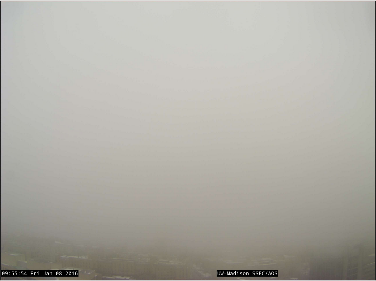
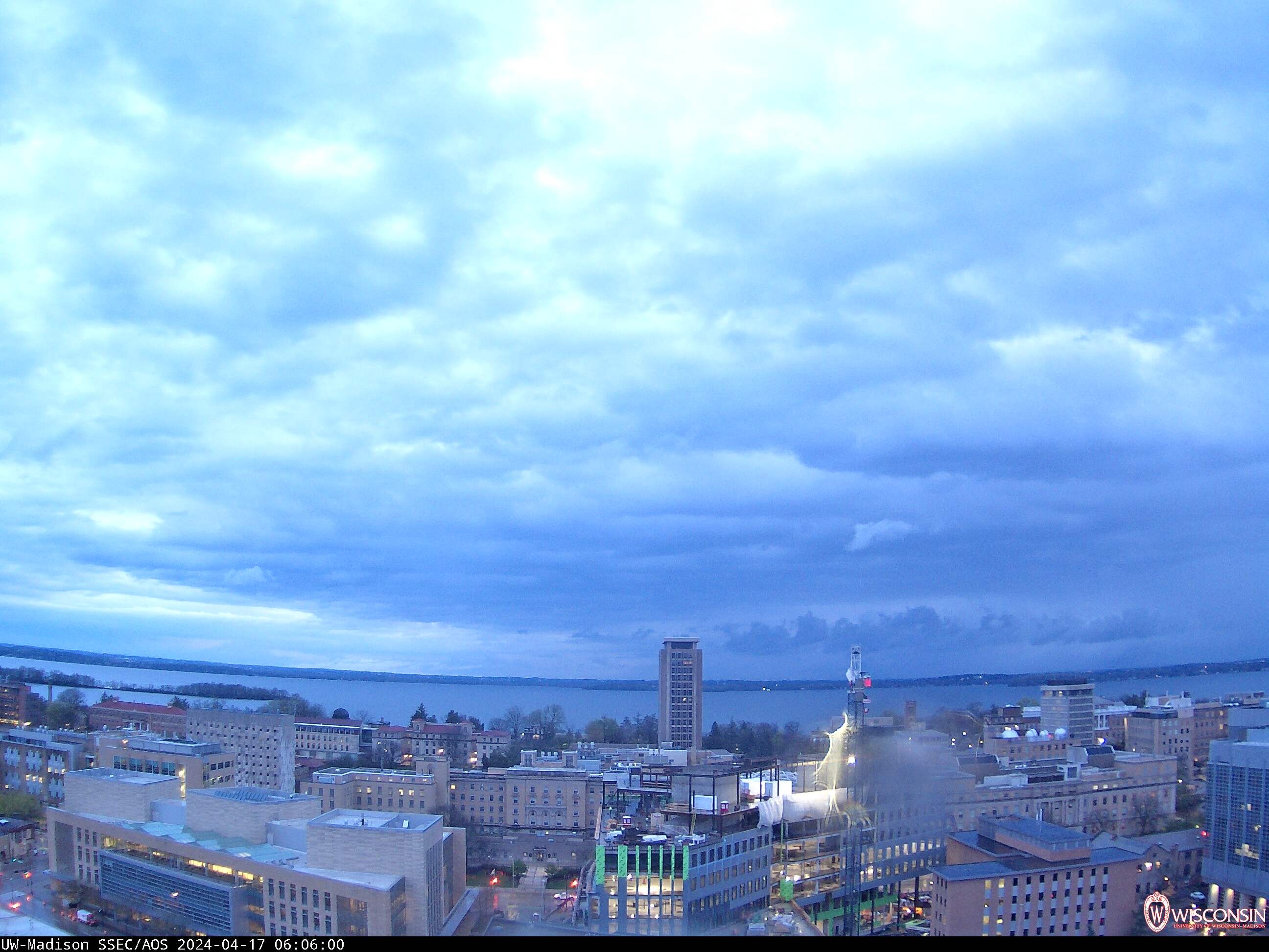
SSEC WebCam, north-facing, at 1555 UTC on 8 January 2016 (Click to enlarge)

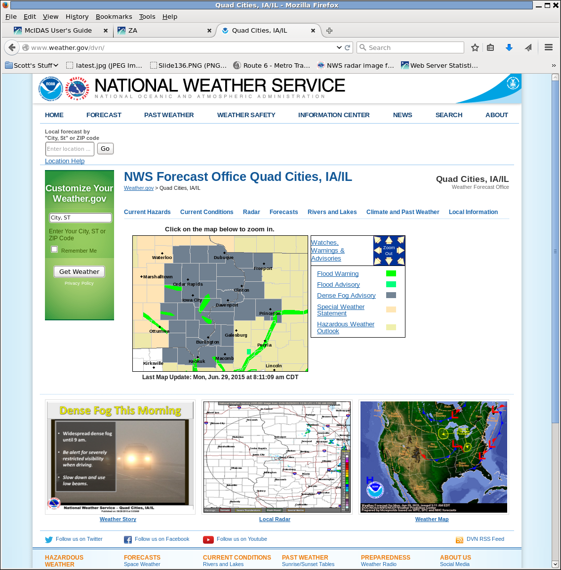
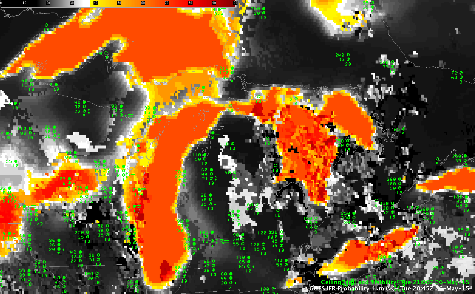
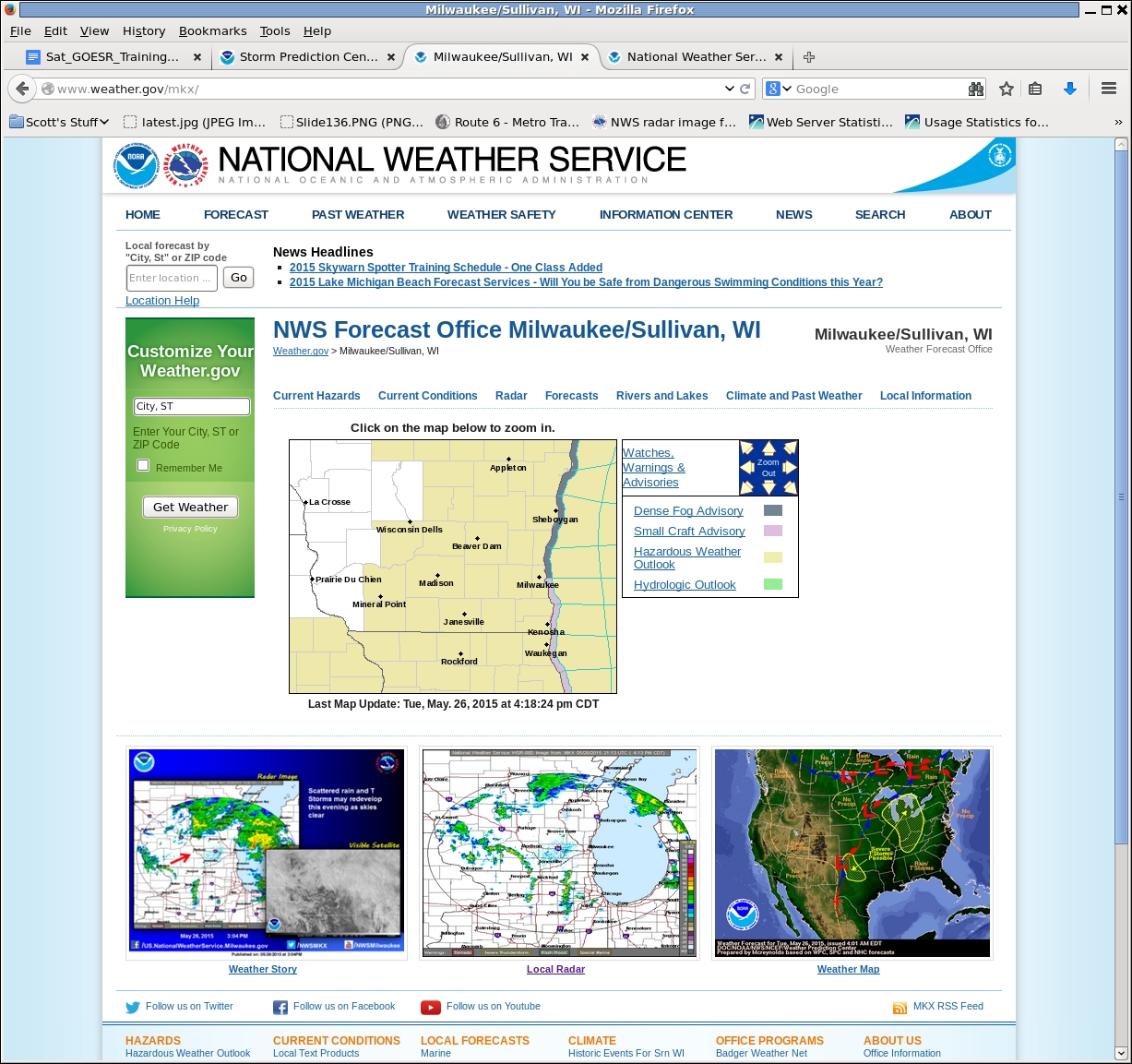
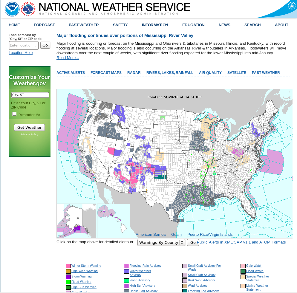
A storm in the Midwest that has drawn moist air northward (dewpoints exceed freezing over snowcover over much of the upper midwest) has caused advection fog over a wide area of the upper midwest. (The WebCam at SSEC in Madison WI (source) is shown above) Dense Fog Advisories (below) were issued by the Davenport, Des Moines, Lincoln and LaCrosse WFOs. Extratropical storm systems are usually accompanied by multiple cloud layers that prevent the satellite from viewing low stratus. For such events as these, only a fog-detection product that includes surface-based information will be useful. GOES-R IFR Probability fields, below, neatly outline the region of lowest visibilities and ceilings. As the highest probabilities push to the east over Wisconsin and Illinois, visibilities and ceilings both drop.

Other aspects of the animation below require comment. IFR Probability fields use predictors based on both satellite and model data; if one of those predictors cannot be used (satellite data, for instance, in regions where high clouds that mask the view of the near-surface), IFR Probability values will be suppressed. The relatively flat nature of the GOES-R IFR probability field over Iowa is characteristic of a field controlled mainly by Rapid Refresh Model output. But there are embedded regions of greater values of IFR Probability that propagate northward: these are regions where breaks in the higher/mid-level clouds allow the satellite to view low clouds, and satellite predictors are available to the algorithm, and probabilities can therefore be larger. Similarly, as the sun rises — at the end of the animation — IFR Probability in general increases as visible imagery can be used for more confident cloud-clearing. The algorithm yield higher probabilities of IFR Conditions because there is more confidence that a cloud is actually present.

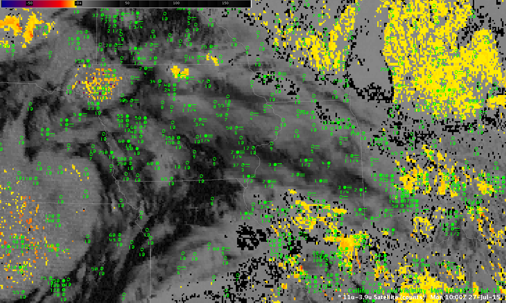
GOES-13 Brightness Temperature Difference values are shown below the IFR Probability field. There is little relationship between the Brightness Temperature Difference field and the reduced surface visibility/lowered ceilings. Note also how the character of the brightness temperature difference field changes as reflected solar radiance becomes important at sunrise.

Hourly GOES-R IFR Probability fields, 0200-1500 UTC on 8 January 2015 (Click to enlarge)

GOES-13 Brightness Temperature Difference (10.7 µm – 3.9 µm) Fields, 0800-1500 UTC on 8 January 2015 (Click to enlarge)

A Blend of Fog and Stratus over the Midwest

GOES-13 Brightness Temperature Difference (10.7 µm – 3.9 µm) fields (color enhanced) and GOES-R IFR Probability fields, and surface observations of ceilings and visibilities, 0200 UTC on 4 December 2015 (Click to enlarge)

Consider the toggle above between GOES-13 Brightness Temperature Difference and GOES-R IFR Probability fields at 0200 UTC on 4 December over the Midwest. (A surface map from 1200 UTC on 4 December shows High Pressure stretched across Ohio and Indiana). IFR Conditions are not reported over Ohio, Indiana or Illinois above. Would you expect them to form? And where? The GOES-R IFR Probability product is distinguishing between low stratus (not quite fog) over Indiana/Illinois and mid-level stratus over Ohio. How do things evolve through the night?

The 0500 UTC image, above, shows IFR conditions reports over south-central Illinois as ceilings lower and visibility degrades under the High Pressure System. By 1000 UTC, below, the IFR Conditions over Illinois are more widespread and near-IFR conditions are present over much of Indiana. Meanwhile, in Ohio, mid-level stratus continues.

By 1215 UTC, IFR conditions have developed over Indiana just before sunrise. Note also the development of IFR conditions along the Ohio River, and that low ceilings did not develop in Michigan (despite the high IFR Probabilities) where winds never relaxed. Use the IFR Probability fields in concert with other observations to make a nearcast/forecast. This case is a good example of using IFR Probabilities as an alert to where IFR conditions may be developing (in addition to the discrimination between low stratus/fog and mid-level fog that is frequently discussed on this blog). IFR Probability can be interpreted as a probability that IFR conditions exist at present or will be existing presently.

Are IFR Conditions Present?

Suomi NPP Visible (0.70 µm) Day Night Band Imagery and Infrared Brightness Temperature Differences (11.45 µm – 3.74 µm), 0731 UTC on 24 November 2015 (Click to enlarge)

Low clouds (with a sharp southern edge) were over northern Wisconsin during the early morning of 24 November 2015. Are IFR Conditions present? Can you tell from the satellite imagery alone? The cloud bank stretched over northern Wisconsin seems thick compared to the bank of clouds over northeastern Wisconsin (centered on southern Green Bay). The city lights of Duluth are not visible in the same way that the city lights of Green Bay are in the Day Night band imagery. Clouds in general are distinct with the near-full moon providing ample illumination.

Both GOES and MODIS Brightness Temperature Difference fields, below, show a signal consistent with low clouds over most of northern WI and adjacent regions. But are there IFR Conditions?

GOES-13 Brightness Temperature Difference (10.7 µm – 3.9 µm) Fields (0730 UTC) and MODIS Brightness Difference Fields (11 µm – 3.9 µm) (0749 UTC)

IFR Probability fields blend the information available from satellite (are water-based clouds present?) with model output to yield a refined diagnostic of IFR Conditions. If there is saturation in the lowest levels (the lowest 1000 feet) of the model, then Probabilities of IFR Conditions are increased. If the lowest levels of the model are relatively dry, in contrast, then IFR Probabilities are reduced. On the morning of 24 November, the latter condition occurred over northern Wisconsin. IFR Probabilities computed from MODIS and GOES-13 satellite values are shown below. Probabilities are very low over most of Wisconsin where mid-level stratus (with varying bases) was present: IFR conditions were not generally observed in the regions where water-based clouds were indicated by the satellite. Mid-level stratus can look, from the top, very similar to fog, but it’s impossible for the satellite alone to discern what’s happening at the cloud base. Model data helps the IFR Probability algorithm screen out regions where mid-level stratus is occurring.

MODIS-based GOES-R IFR Probabilities (0751 UTC), GOES-13-based GOES-R IFR Probabilities (0731 UTC), and GOES-based GOES-R IFR Probabilities with surface observations of ceilings and visibilities (Click to enlarge)

Widespread Fog over the central United States

GOES-R IFR Probability Field and GOES-13 Brightness Temperature Difference (10.7µm – 3.9µm) at 1145 UTC on 3 November 2015. Surface-based observations of ceilings and visibilities are plotted (Click to enlarge)

Fog was widespread over the central United States on the morning of 3 November, and Dense Fog Advisories were commonplace. The toggle above compares the Brightness Temperature Difference field (10.7 µm – 3.9 µm) with the GOES-R IFR Probability field at 1145 UTC on 3 November. (This toggle is much faster) IFR Probabilities use near-surface information in the Rapid Refresh Model to screen out regions where Brightness Temperature Difference signals are showing elevated stratus rather than fog (For example, the region around Columbus MS). IFR Probabilities are also low in regions with a modest brightness temperature difference return (most of eastern Nebraska, west Texas, southern Indiana along the Ohio River); these regions do not include stations observing IFR Conditions.

Fog under high clouds in Indiana

GOES-R IFR Probability (Upper Left), GOES-R Low IFR Probability (Lower Left), GOES-13 Brightness Temperature Difference (10.7µm – 3.9µm) (Upper Right), GOES-R Cloud Thickness (Lower Right) (Click to enlarge)

Fog developed over Indiana and surrouding states (again) on the morning of 6 October, and the animation above traces that development as diagnosed by GOES-R IFR Probability fields. Multiple cloud layers over the region meant that the Brightness Temperature Difference field, a traditional method of low cloud detection (that keys on the differences in emissivity at 10.7 and 3.9 in water-based clouds) could not be used because low cloud detection was hampered by the presence of high clouds. The fused product, GOES-R IFR Probability, provides useful information by combining Rapid Refresh Data information about low-level saturation with satellite fields. When satellite information about low clouds are missing, as in this case, model data provides a signal.

Because multiple cloud layers exist, the GOES-R Cloud Thickness Product (that diagnoses the depth of the lowest water-based cloud based on an empirical relationship between 3.9 µm emissivity and cloud depth developed using sodar observations off the West Coast of the United States) is not produced over much of the region. It is also not produced at times of twilight — such as those that occur at the end of the animation. There are values over southeastern lower Michigan at the start of the animation, where high clouds were not present.

Low IFR Probability is also shown in the animation above (Lower Left figures). The small values in this case suggest any fog is unlikely to be producing visibilities less than 1 mile or ceilings less than 500 feet.

IFR Probability across the Midwest under cirrus

Midwest_1000_1215_27July2015_GOES13_IFRPROBanim

GOES-R IFR Probability fields, 1000, 1115 and 1215 UTC on July 27 2015 along with surface plots of ceilings and visibility (Click to enlarge)

Regions of dense fog developed over the Midwest during the morning of July 27 2015, and the GOES-R IFR Probability fields are shown above for 1000 through 1215 UTC. There is a good spatial relationship to where IFR Probabilities are large(ish) and where IFR conditions are present. This example is a good reminder that GOES-R IFR Probability fields should be interpreted with knowledge of other fields. On this day, an extensive cirrus shield (Click the link to view the Brightness Temperature Difference field at 1000 UTC) prevented GOES-13 from viewing low clouds over much of the midwest; thus, the IFR Probability field was driven mostly by model fields over Illinois and Iowa. This is why the field there is mostly uniform. When satellite data is not used in computing the probabilities (because of cirrus clouds), the magnitude of the IFR Probability is reduced.

Fog over Iowa

GOES-R IFR Probability fields, 0400-1215 UTC, 20 July 2015 (Click to enlarge)

Dense fog developed over portions of eastern Iowa early in the morning of 20 July 2015. The animation above shows the hourly evolution of the GOES-R IFR Probability fields computed using satellite data from GOES-13 and Rapid Refresh model output. The flat nature of the fields in the animation above suggests the satellite data cannot view the near-surface because of higher level clouds; Brightness Temperature Difference fields, below, from 0615, 0800 and 1000 UTC confirm that hypothesis. This was a case where inclusion of the Rapid Refresh information was vital for the IFR Probability field to outline correctly the region of visibility restrictions due to fog. Note that the last GOES-based GOES-R IFR Probability image, at 1215 UTC, above, after sunrise, shows a general increase in values over the 1100 UTC image (just before sunrise). Daytime predictors (used here at 1215 UTC) result in a higher probability of IFR conditions that nighttime predictors (used here at 1100 UTC) in part because of the use of visible data for cloud-clearing.

GOES13_BTD_20July2015_0615_0800_1000step

GOES-13 Brightness Temperature Difference fields (10.7µm – 3.9µm) at 0615, 0800 and 1000 UTC on 20 July 2015 (Click to enlarge)

An Aqua overpass provided MODIS information at ~0830 UTC, and toggle between the brightness temperature difference field (11.0µm – 3.7µm) and MODIS-based IFR Probabilities, below, shows MODIS-based IFR Probabilities were enhanced over southern and eastern Iowa in a region where the brightness temperature difference field gave a signal consistent with mid- and high-level clouds.

Aqua MODIS Brightness Temperature Difference (11.0µm – 3.7µm) and MODIS-based GOES-R IFR Probabilities, ~0830 UTC on 20 July 2015 (Click to enlarge)

MODIS-based vs. GOES-based IFR Probabilities

The CIMSS Satellite Blog shows a case on July 2nd 2015 of Day Night Band detection of river valley fog over the upper midwest. River Valley fog is a challenge for GOES detection because of the large pixel footprint. So how did it do in this case, and how does that compare to MODIS-based detection? The animation below shows the three MODIS scenes during fog development that occurred. MODIS-based IFR Probability at 0432 UTC (from Terra) hints at the development of fog over the Wisconsin and Kickapoo Rivers over southwestern WI. GOES-based IFR Probability from 0430 UTC (shown below the MODIS data) shows no signal there. GOES-based IFR Probabilities do appear at 0715 UTC, however. The MODIS-based signal has given any forecaster an early alert to the development of fog over the River valleys. (Toggles between GOES and MODIS-based IFR Probabilities are available for 0430 UTC, 0715 UTC and 0845 UTC). Note that both 0710 and 0848 UTC MODIS-based fields (from Aqua) have a geometry such that the Mississippi River valley is near the edge, and artifacts related to the so-called bow-tie effect are present as repeated features in the field. Nevertheless, the MODIS-based field correctly limits the fog to the River Valleys and shows very high IFR Probabilities; GOES-based pixels fail to resolve narrow river valleys.

MODIS-based GOES-R IFR Probabilities, 0432, 0710 and 0848 UTC on 2 July 2015 (Click to enlarge)

GOES-based GOES-R IFR Probabilities, 0430, 0715 and 0845 UTC on 2 July 2015 (Click to enlarge)

An animation of GOES-based IFR Probabilities, below, suggests that GOES data identified the likelihood of IFR conditions starting around 0515 UTC, almost 45 minutes after the higher-resolution MODIS pass at 0432 UTC.

GOES-based GOES-R IFR Probabilities, 0430 – 0545 UTC on 2 July 2015 (Click to enlarge)

Dense Fog over Iowa and Illinois

Front page of the National Weather Service in the Quad Cities, Monday morning 29 June 2015 (Click to enlarge)

Dense fog developed over the mid-Mississippi Valley early on Monday, 29 June 2015, and Dense Fog Advisories were hoisted by the DVN WFO, as shown above. How did the GOES-IFR Probabilities (and other products) capture this event? The animation below shows the evolution of surface visibilities at 0600, 0800 and 1000 UTC. IFR Conditions have developed by 0600 UTC and they subsequently expand.

Surface Visibilities (Statute Miles) over Iowa, 0600, 0800 and 1000 UTC, 29 June 2015. IFR Conditions are highlighted in white (Click to enlarge)

The Day Night band suggests clouds are present over parts of Iowa at 0707 UTC, but the waxing gibbous moon has set by 0848 UTC (below), and the lack of reflected moonlight at the later time precludes cloud detection. The brightness temperature difference (11.45µm – 3.74µm) from Suomi NPP can detect the tops water-based low clouds and it does confirm that the clouds have not vanished at 0848 UTC despite the lack of signal in the Day Night band. The brightness temperature difference field includes signals (black in the enhancement used) that suggest the presence of cirrus clouds.

VIIRS_DNB__REF_20150629_toggle_0707_0848

Visible Imagery from the Suomi NPP Day Night Band, 0707 and 0848 UTC on 29 June 2015 (Click to enlarge)

Suomi NPP Brightness Temperature Difference (11.45µm – 3.74µm) at 0707 UTC and 0848 UTC (Click to enlarge)

MODIS data can be used to compute IFR Probability fields. These fields are not available frequently, although they do present a high-resolution view of events when available. Two overpasses, at 0408 (Terra) and 0817 (Aqua), provided imagery early on 29 June. The MODIS data suggests the development of a large area of fog. What does GOES data show? Click here for a comparison of MODIS and GOES at 0408 UTC, and here for a comparison of MODIS and GOES at 0817 UTC). The chief difference between MODIS and GOES is somewhat higher values at the earlier time, and sharper edges (as might be expected given the resolution differences) at both times.

MODIS-based GOES-IFR Probabilities, 0408 and 0817 UTC on 29 June 2015 (Click to enlarge)

GOES-R IFR Probabilities computed from GOES-13 have a temporal resolution that allows for monitoring of fog development, and values increase rapidly after 0500 UTC over eastern Iowa, in accord with the development of IFR observations shown above. Brightness Temperature Difference fields (bottom) also suggest the development of low clouds over Iowa. However, there are places where high clouds prevent a signal and the rising sun (and its 3.9 µm radiation) mean the signal is reduced at the end of the animation. GOES-R IFR Probabilities maintain a coherent signal through sunrise.

GOES-based GOES-R IFR Probabilities, 0400-1215 UTC on 29 June 2015 (Click to enlarge)

GOES-13 Brightness Temperature Difference (10.7 µm – 3.9 µm), 0400-1215 UTC, 29 June 2015 (Click to enlarge)

Late Spring in the Great Lakes: Fog

GOES-R IFR Probability fields, 2100 UTC on 26 May 2015, along with surface observations of ceilings and visibility (Click to enlarge)

Sea or lake surface temperatures are part of the algorithm used to create IFR Probability fields. The cold Great Lakes in late May are a prime location for advection fog, and IFR Probability fields will blanket the Great Lakes with high values under southerly, moist flow. It is not uncommon to see all of the Lakes bright orange/red. Note in the image above how Manitowoc WI and Charlevoix MI both have IFR Conditions. In addition, Dense Fog advisories were issued north of Milwaukee to the tip of Door County.

GOES-R Fog Product Examples

Fog detection fusing GOES, Terra/Aqua or Suomi/NPP Satellite data with Model output