Category Archives: Midwest

Cloud Thickness and Dissipation Time

goes-rcloudthickness_1130utc_20sept2016

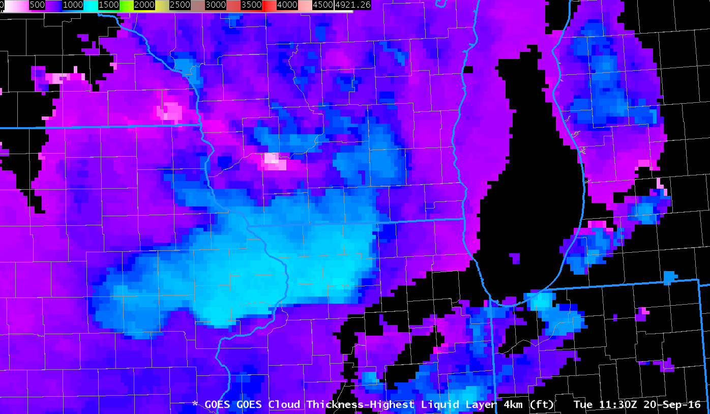
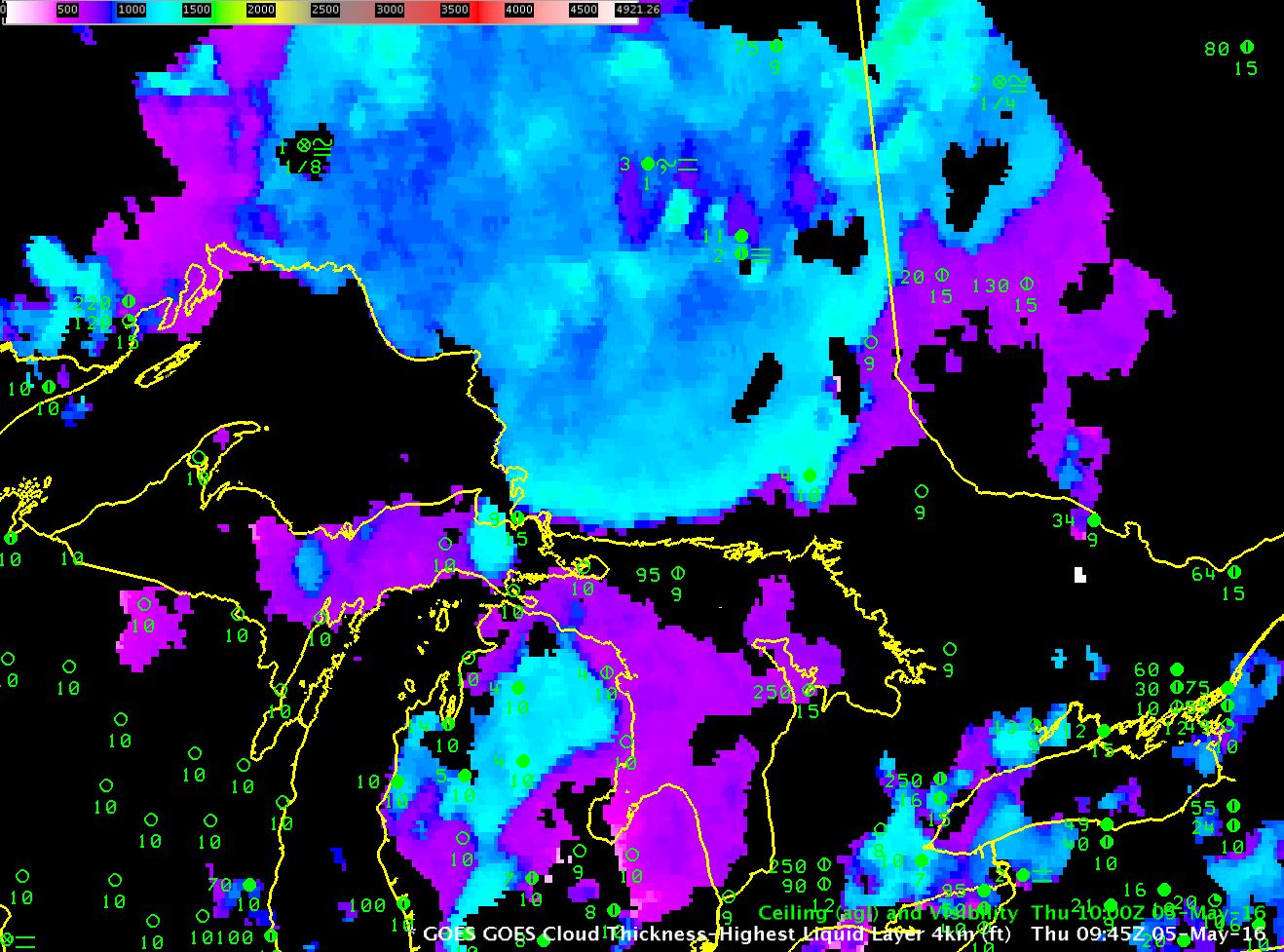
GOES-R Cloud Thickness Fields, 1130 UTC on 20 September 2016 (Click to enlarge)

GOES-R Cloud Thickness is created from a look-up table created from observations of 3.9 µm emissivity and sodar observations of cloud thickness off the west coast of the United States.  The product is not computed during twilight conditions when rapid changes in reflected solar radiation (either increases around sunrise or decreases around sunset).  The image above shows the GOES-R Cloud Thickness field over the midwest just before sunrise on 20 September 2016 (Radiation fog formed subsequent to late-afternoon and evening thunderstorms over Wisconsin and Illinois).  This scatterplot relates the last pre-sunrise value to dissipation time.  GOES-R Cloud thickness shows values over the Wisconsin River Valley in southwest Wisconsin, and over regions south of Military Ridge. Largest values — 1100 feet over Illinois and Iowa — suggest (from the scatterplot) a dissipation time of around 4 hours, which would be 1130 UTC (the time of the image) + 4 hours, or 1530 UTC.  There is also a region of thick clouds on northwest Indiana on the shore of Lake Michigan.  It’s these regions where you should expect large-scale fog/low clouds to dissipate last.   The animation below shows that to be true.  Fog over the river valleys is taking a bit longer to dissipate than expected, however. Note: navigation in the animation shows the effect of the loss of one star-tracker on GOES-13.

goes13_flswi_20sept2016_1245_1515anim

GOES-13 Visible (0.63 µm) animation, 1245-1515 UTC on 20 September 2016 (Click to enlarge)

The Day Night band on the VIIRS instrument on board Suomi NPP produces visible imagery at night that showed the regions of fog distinctly shortly after 0800 UTC on 20 September as shown below.

daynightband_wi_0827_20sep2016

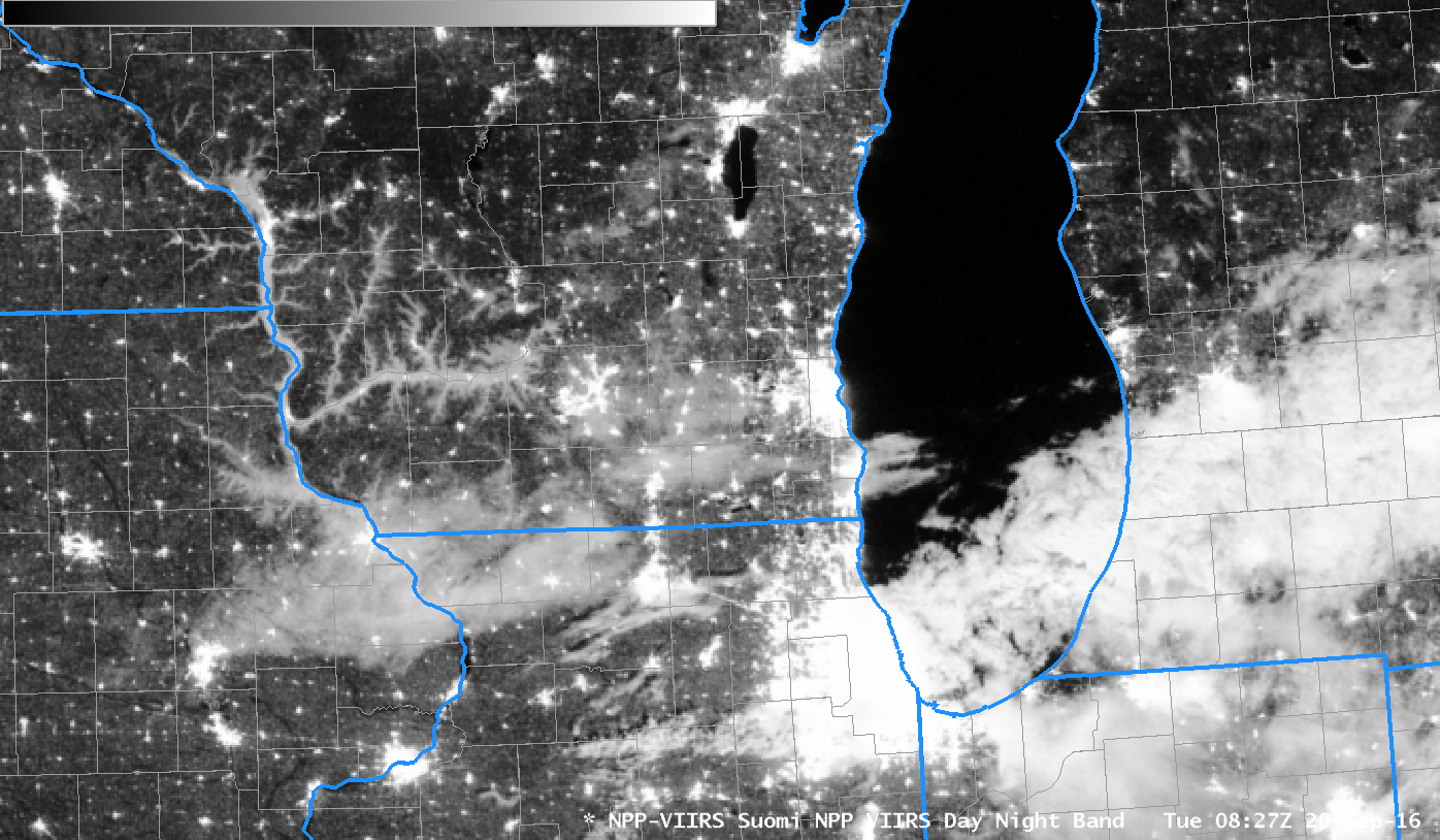
VIIRS Day/Night Band Visible (0.70 µm) Imagery from Suomi NPP at 0827 UTC on 20 September (Click to enlarge)

Fog under High Clouds

FourPanel_1045UTC_18August2016

GOES-R IFR Probability Fields (Upper left), GOES-East Brightness Temperature Difference (3.9 – 10.7) (Upper Right), GOES-R Cloud Thickness (Lower Left) and GOES-East Water Vapor imagery (Lower Right), all at 1045 UTC on 18 August 2016. Surface observations of ceilings and visibilities at 1100 UTC are included in the upper right (Click to enlarge)

Dense Fog developed over southern Indiana on the morning of August 18 (and advisories were hoisted).  The single image above demonstrates an advantage of GOES-R IFR Probability fields in determining the areal extent of fog:  the traditional method of night-time fog detection from satellite fails in regions where cirrus clouds obscure the view of low clouds.  That was the case over the Ohio River Valley where IFR conditions were occurring.  GOES-R IFR Probability fields have a signal where high clouds exist in regions where Rapid Refresh model output shows low-level saturation, as over southwestern Indiana.  Because satellite data cannot be used there to compute IFR Probabilities, the magnitude of the probability is smaller.  Tailor your interpretation of the IFR Values based on the presence of high clouds.  The presence of high clouds changes the character of the IFR Probability field, from a pixelated field where satellite data are present to a flatter field where only model data can be used.

GOES-R Cloud Thickness can be used to estimate fog dissipation time (using this scatterplot, where the thickness values are from the last pre-sunrise scene).  That field, however, is only produced where the satellite has an unimpeded view of the low clouds (therefore, where cirrus clouds are present, as over the Ohio River Valley, Cloud Thickness is not produced).   Note the line parallel to the terminator over eastern Ohio:  GOES-R Cloud Thickness is not produced during twilight times around sunrise or sunset.  This 1045 UTC image is the final one over Indiana before sunrise.  Maximum thickness values are just over 1000 feet over southwest Indiana, suggesting a dissipation time of about three hours, that is, around 1345 UTC.

Changes in Model Fields show up in IFR Probability

GOES-R_IFR_1045_1100UTC_15August2016toggle

When GOES-R IFR Probability fields are governed solely by Rapid Refresh model output because of thick cloudiness (as was the case over Illinois on 15 August 2016), there can be changes in the field at the top of the hour that are related to changes in the Rapid Refresh model output — that is, changes in which hour Rapid Refresh Model is used.  The toggle above shows the IFR Probability fields at 1045 UTC and 1100 UTC on 15 August.  Both fields are characterized by smooth values that come with IFR Probability that is driven by Rapid Refresh model output, output that is smooth and not pixelated like satellite data.  It’s pretty noticeable, however, that values increase (from ~39% to ~52%) in those 15 minutes.  Why?

The image below shows Rapid Refresh Model Predictions of 1000-700 mb Relative Humidity at 1100 UTC from the 0800 UTC model run (that is, a 3-hour forecast, left) and from the 0900 UTC model run (that is, a 2-hour forecast, right).  Relative Humidity Values from the 0800 UTC Run (interpolated to 1045) are used in the computation of IFR Probabilities at 1045 UTC;  values from the 0900 UTC Run are used in the computation of IFR Probabilities at 1100 UTC.  It’s not this relative humidity field (value from 1000-700 hPa) precisely that is used, but rather maximum values in the vertical.  Certainly there are changes in the predicted low-level relative humidity field at 1100 UTC between the sequential model runs;  it’s more likely that saturation is occurring in the later model run, and that greater likelihood of saturation is reflected in the change of IFR Probability from 1045 UTC (when 0800 UTC Rapid Refresh Model fields are used) to 1100 UTC (when 0900 UTC Rapid Refresh Model fields are used).

RAP_RH_11UTC_15AUG2016

Rapid Refresh model predictions of 1000-700 mb Relative Humidity; 3-hour forecast from the 0800 UTC Rapid Refresh Model (left) and 2-hour forecast from the 0900 UTC Rapid Refresh Model (Right), both from 15 August 2016 (Click to enlarge)

Dense Fog over Missouri and Illinois

Dense Fog Advisories were issued before sunrise on 5 July 2016 by the National Weather Service Offices in St Louis Missouri and Lincoln Illinois (link).  This post compares GOES-R IFR Probability fields with Brightness Temperature Difference Fields for that event.  At 0500 UTC, the Brightness Temperature Difference Field had a very strong signal over central/northern Illinois.  This region of mid-level stratus was de-emphasized by the GOES-R IFR Probability fields because of a lack of low-level saturation in the Rapid Refresh Model Fields.  At 0500 UTC, IFR Probability Fields show an increase in values over the lower Ohio River Valley.

GOES_BTD_IFRP_0500_05July2016toggle

GOES-13 Brightness Temperature Difference Field (3.9 µm – 10.7 µm) and GOES-R IFR Probability Fields, 0500 UTC on 5 July 2016 (Click to enlarge)

At 0700 UTC, below, an axis of higher probabilities has developed northwest to southeast across central Missouri;  in addition, IFR Probabilities are increasing slowly over central Illinois to the south of the mid-level stratus that persists over east-central parts of Illinois.  IFR Conditions are present at stations over central Illinois  (Springfield — KSPI — and Litchfield — K3LF, for example)

GOES_BTD_IFRP_0700_05July2016toggle

GOES-13 Brightness Temperature Difference Field (3.9 µm – 10.7 µm) and GOES-R IFR Probability Fields, 0700 UTC on 5 July 2016 (Click to enlarge)

By 1000 UTC, below, when Dense Fog Advisories have been issued, a strong brightness temperature difference signal is present over much of northern Missouri, but mid-level clouds over southeast Missouri prevent a strong signal from occurring there where fog is occurring.  IFR Probability Fields’ use of Rapid Refresh information mitigates this lack of satellite observations.    IFR Probability fields at 1000 UTC show a signal over much of southern Illinois where IFR Conditions are widespread.

GOES_BTD_IFRP_1000_05July2016toggle

GOES-13 Brightness Temperature Difference Field (3.9 µm – 10.7 µm) and GOES-R IFR Probability Fields, 1000 UTC on 5 July 2016 (Click to enlarge)

Use IFR Probability fields as a tool to become situationally aware to the development of lowered ceilings and reduced visibilities.  There are many times when Brightness Temperature Difference fields cannot tell the entire story — when multiple cloud layers exist, for example, or when mid-level stratus is present. A slow increase in GOES-R IFR Probability will often suggest lowering ceilings/reduced visibilities before Brightness Temperature Difference fields do.

Low Ceilings and reduced visibilities over the Ohio Valley

1200UTC_OhioValley24June2016

Surface Observations at 1200 UTC on 24 June 2016 (Click to enlarge)

A screen capture from this site at 1215 UTC on 24 June 2016, above, shows IFR Conditions (Red) and Low IFR Conditions (Purple) over the upper Ohio River Valley and surrounding states.  The IFR Probability field for the same time, below, shows high probabilities in roughly the same regions that have IFR or Low IFR conditions.  The Brightness Temperature Difference field, also displayed in the toggle below, gives little information at this time of day.  A benefit of the GOES-R IFR Probability field is that it contains a coherent signal through sunrise.

GOES_IFR_BTD_1215_24June2016toggle

GOES-R IFR Probability fields and GOES-13 Brightness Temperature Difference Fields (3.9 µm – 10.7 µm) at 1215 UTC on 24 June 2016 (Click to enlarge)

The toggle at 0915 UTC, below, before sunrise, shows a second benefit of IFR Probability fields: a useful signal in regions with cirrus clouds. High clouds, of course, prevent GOES-13 from viewing the development of fog/low stratus near the surface. The Rapid Refresh model data on low-level saturation that are part of the IFR Probability Field computations give quality information in regions of cirrus. In the example below, developing IFR conditions are depicted (the yellow enhancement that shows IFR Probabilities around 40%) over much of northern Kentucky and southern Ohio.  This is under a region of cirrus (black in the enhancement used for the brightness temperature difference) north of a convective system that sits over southeastern Kentucky and eastern Tennessee.

GOES_IFR_BTD_0915_24June2016toggle

GOES-R IFR Probability fields and GOES-13 Brightness Temperature Difference Fields (3.9 µm – 10.7 µm) at 0915 UTC on 24 June 2016 (Click to enlarge)

The waning full moon provided ample illumination for the Suomi NPP Day/Night Band Imagery, shown below, from 0736 UTC on 24 June 2016.  The cirrus shield, mid-level clouds and developing valley fogs are all apparent.

NPP_DNB_0736_24June2016

Suomi NPP Day/Night band imagery, 0736 UTC on 24 June 2016 (Click to enlarge)

For over the Northern Plains

IFRProb_0215_1115_01June2016anim

GOES-R IFR Probability Fields, computed from GOES-13 and Rapid Refresh output, 0215-1115 UTC on 1 June 2016 (Click to enlarge)

Dense Fog Advisories were issued over parts of Iowa and Minnesota early on 1 June 2016 (see map below). The fog developed over wet ground left in the wake of convection that moved through the region late in the day on 30 May/early on 1 June (Precipitation totals available here).  GOES-R IFR Probability fields, above, show the two areas of dense fog developing.  The region over Minnesota was characterized a lack of high clouds — the satellite could view the developing fog, and satellite parameters were included in the computation of IFR Probability.  Consequently, the IFR Probability values were larger.

Fog over Iowa initially developed under mid-level clouds behind departing convection. IFR Probability fields in that case show a flatter distribution because horizontal variability is controlled mostly by model fields that are smooth; additionally, IFR Probability values are somewhat reduced because satellite predictors cannot be used. By 0815 UTC, however, mid- and high-level clouds have dissipated, and the satellite has a unobstructed view of the fog/stratus. Satellite predictors could then be used and IFR Probabilities increased, and the field itself shows more horizontal variability as might be expected from the use of nominal 4-km resolution satellite pixels.

weather.gov

Screen Capture of weather.gov website at 1129 UTC on 1 June. Dense Fog Advisories are indicated over eastern Iowa and northeast Minnesota (click to enlarge)

Cloud Thickness and Dissipation Time

CloudThickness_0945_05May2016

GOES-R Cloud Thickness, 0945 UTC on 5 May 2016. Note that Cloud Thickness is not computed in the northeast corner where twilight has begun. This is last scene for northern Ontario and Michigan. (Click to enlarge)

GOES-R Cloud Thickness can be used to make a first guess of when fog and low clouds will dissipate. This is done via a look-up table that is derived from this scatterplot. The y-axis on that plot is the last GOES-R Cloud Thickness field produced before sunrise, such as that shown above, and the x-axis is the number of hours after the plot that clearing is expected, GOES-R Cloud Thickness relates 3.9 µm emissivity to dissipation time based on SODAR observations from off the West Coast, and the scatterplot was derived mostly from observations over the southeast US;  the thickness is that of the lowest water-based cloud field and it’s not computed where multiple cloud layers exist — near Geraldton north of Lake Superior, for example, where IFR Conditions are reported — or near sunrise/sunset.  Values are between 1100 and 1200 feet over northern Lower Michigan,  around 1200 feet over eastern upper Michigan, and around 1200 to as much as 1490 feet over northwest Quebec.  The scatterplot suggests a dissipation time of nearly 4 hours, which would be 1345 UTC.

Imagery below shows low clouds persisting just past 1500 UTC.  For this region where the sun angle is not as high as over the southeast US (where most of the observations used for the scatterplot creation were taken), burn-off took a bit longer.  However, note that GOES-R Cloud Thickness did highlight the thickest clouds that took the longest to dissipate;  so, although the scatterplot underestimated the time of dissipation, Cloud Thickness values did identify which regions would clear last.

A final note: GOES-R Cloud Thickness Dissipation times were computed for Radiation Fog Events, such as the one on 5 May 2016. Dissipation of other fogs that create IFR conditions — Advection Fog, Tule Fog — will not be forecast well with this technique.

GOES13VISLoop_1115_1515_5May2016

GOES-13 Visual (0.63 µm) imagery, 1115-1515 UTC on 5 May 2016 (Click to enlarge)

Low Ceilings and Reduced Visibilities over the Upper Midwest

IFRP_0515_1315anim

GOES-R IFR Probability, 0515-1315 UTC on 26 April, with surface observations of ceilings and visibility (Click to enlarge)

GOES-R IFR Probability fields, above, expand southwestward across the upper midwest as ceilings lower and visibilities reduce.  The fields offered quick guidance on where the lowest ceilings were occurring and how the field of low clouds was evolving.  After sunrise (1215 and 1315 UTC imagery), IFR Probability values increased but continued to show a coherent signal over the region of lowest ceilings and smallest visibility.

The Brightness Temperature Difference fields for the same times, below, have structures that have echoes in the IFR Probability fields. The depiction of low ceilings and visibilities associated with the largest brightness temperature difference values (the deepest orange-red in the enhancement) is lost, however, as reflected 3.9 µm radiation alters the brightness temperature difference field. By 1315 UTC, the end of the animation, only the IFR Probability field is giving useful information about the low ceilings and reduced visibilities.

BTD_0515_1315anim

GOES-13 Brightness Temperature Difference (10.7 µm – 3.9 µm) Fields, hourly from 0515 through 1315 UTC, 26 April 2016 (Click the enlarge)

Widespread IFR conditions over the Upper Midwest

GOESR_IFRP_0215_1215stepanim

GOES-R IFR Probability Fields, hourly from 0215-1215, 14 March 2016 (Click to enlarge)

A rain-dampened boundary layer allowed fog to form over much of the upper midwest on early Monday March 14 2016 (as a baggy low pressure system moved eastward). GOES-R IFR Probability fields, above, captured the slow expansion of the region of IFR conditions.  The character of the IFR Probability Field varies from smooth (over northern Illinois at 0215 UTC, for example (link)) to pixelated (over southern Minnesota at the same time).  This is related to whether the model only is used as a predictor (over northern Illinois) because of high clouds that prevent the satellite from viewing low clouds or whether model and satellite data are both used as predictors (over southern Minnesota).  The toggle below, of IFR Probability Fields and Brightness Temperature Difference fields at 1000 UTC on 14 March, underscores this relationship between IFR Probability and Brightness Temperature Difference fields.

In the animation above, IFR conditions are in general observed where IFR Probability fields suggest their presence.

GOES_IFR_BTD_14March2016_1000ztoggle

GOES-R IFR Probability and GOES-13 Brightness Temperature Difference Field, 1000 UTC on 14 March 2016 (Click to enlarge)

Fog over the Tennessee River Valley

IFRP_0115_1315stepanim_17Feb2016

GOES-R IFR Probability fields, every two hours from 0115 through 1315 UTC on 17 February 2016 (Click to enlarge)

GOES-R IFR Probability fields showed large values over parts of Kentucky and Tennessee during the overnight hours on 16-17 February 2016, as shown in the animation above (every 2 hours from 0115 through 1315 UTC). (IFR or near-IFR Conditions were present over the region of enhanced IFR Probabilities) For much of the overnight hours, mid-level and high clouds prevented an unobstructed satellite view of low clouds, so Rapid Refresh model output was the principle driver in IFR Probabilities. When that happens, the character of the IFR Probability field is less pixelated (it’s a flatter field) and values are smaller. At the end of the animation — 1315 UTC — satellite observations of low clouds have improved and the GOES-R IFR Probability field is (1) more pixelated, as expected when satellite data are used and (2) showing higher values because Satellite Predictors can be used in the computation of IFR Probability.

MODIS data from Terra and Aqua satellites can also be used to compute IFR Probability fields, and the high spatial resolution of the MODIS instrument (1-km vs. nominal 4-km on GOES) can yield superior results for valley fogs, for example (The effects of some rivers are apparent in the 0354 UTC image over western Tennessee, for example). For a large-scale event as above, however, GOES-based resolutions can be adequate. The toggle of MODIS-based GOES-R IFR Probabilities at 0354 UTC and 0810 UTC is shown below. Patchy clouds (that prevent MODIS from viewing low clouds) are more apparent in the 0354 UTC image than in the 0810 UTC image.

MODIS_IFRP_0354_0810UTC_17Feb2016toggle

MODIS-based GOES-R IFR Probabilities, 0354 and 0810 UTC on 17 February 2016 (Click to enlarge)

Suomi NPP Overflew the Tennessee River valley just after midnight local time, and the toggle of the Day Night band and the Brightness Temperature Difference field (11.45 – 3.74) is shown below. Extensive cloud cover is apparent. The importance of the IFR Probability fields is that it incorporates surface information (from the Rapid Refresh predictions of saturation in the lowest 1000 feet of the model atmosphere) so that fog and low stratus that impacts transportation by reducing visibilities can be distinguished from mid-level stratus that has a smaller impact.

SNPP_DNB_BTD_0735UTC_17Feb2016toggle

Suomi NPP Brightness Temperature Difference fields (10.8 µm – 3.74 µm) and Day Night band visible imagery (0.70 µm) at 0735 UTC on 17 Feburary 2016 (Click to enlarge)