Category Archives: California

Central Valley Fog under High Clouds

A potent storm in the Gulf of Alaska (Link to surface map) is allowing high clouds to spread inland over much of the west coast of the United States. Dense fog has formed underneath that cloud deck in the California’s Central Valley, and advisories have been issued (Scroll down to see the screen-grab of the NWS Sacramento Office Website). How can satellite products be used to detect such a fog that is hidden by high clouds?

The toggle below shows the GOES-15 Brightness Temperature Difference fields (with a pattern characteristic of mostly high (ice) clouds with a few breaks in the high cloud allowing the satellite to view lower water-based clouds) and the GOES-R IFR Probability field. IFR Probability is correctly alerting any forecaster to the probability that IFR conditions are occurring in the Central Valley. IFR Probability fuses information from the Satellite (not particularly helpful in this case) and information from the Rapid Refresh Model predictions of low-level saturation. The Rapid Refresh is correctly diagnosing the presence of saturation, and IFR Probabilities are enhanced over the Central Valley.

GOES-15 Brightness Temperature Difference and GOES-R IFR Probability fields, 1115 UTC on 8 December 2015 (Click to enlarge)

Coastal California Fog

Toggle between Suomi NPP Day Night Band Visible (0.70 µm) Image and Brightness Temperature Difference (11.45 µm – 3.74 µm) , 1003 UTC 12 August 2015 (Click to enlarge)

Suomi NPP data from 1003 UTC on 12 August, above, shows evidence of a cloud bank hugging the northern California coast from Cape Mendocino to San Francisco Bay. It also penetrates inland to Santa Rosa in Sonoma County. (Note also how the fires burning in interior show up well in the Day Night Band — they are emitting visible light — and in the Brightness Temperature Difference band — because they are much warmer in the 3.74 µm image than in the 11.45 µm image).

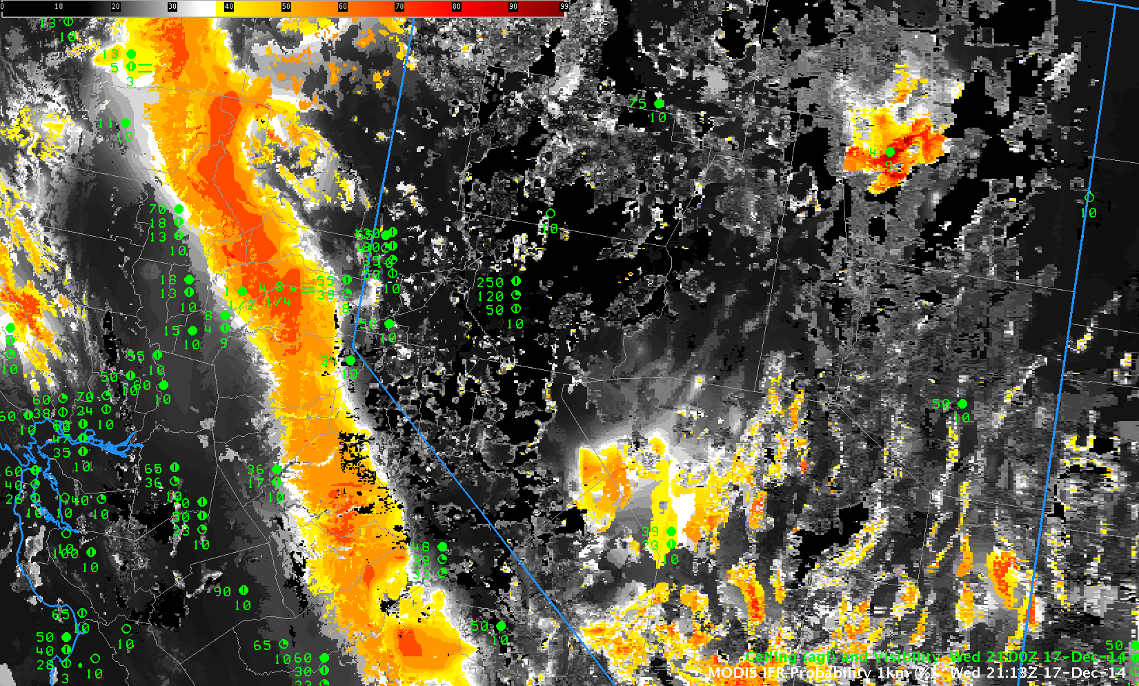
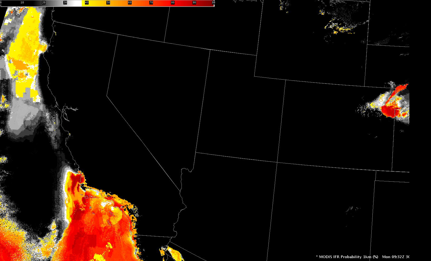
Terra overflew the California coast at ~0600 UTC and Aqua overflew the coast at ~1000 UTC; MODIS-based IFR Probabilities could be constructed from these overpasses, and they are shown below. At 0609 UTC, High IFR Probabilities (>90%) are confined to coastal Sonoma County and along the coast from Humboldt county north. By 1023 UTC, high IFR Probabilities stretch along the entire coast from Cape Mendocino to the mouth of San Francisco Bay, with evidence of inland penetration along river valleys. (The Russian River, for example, and perhaps the Noyo River in Mendocino County)

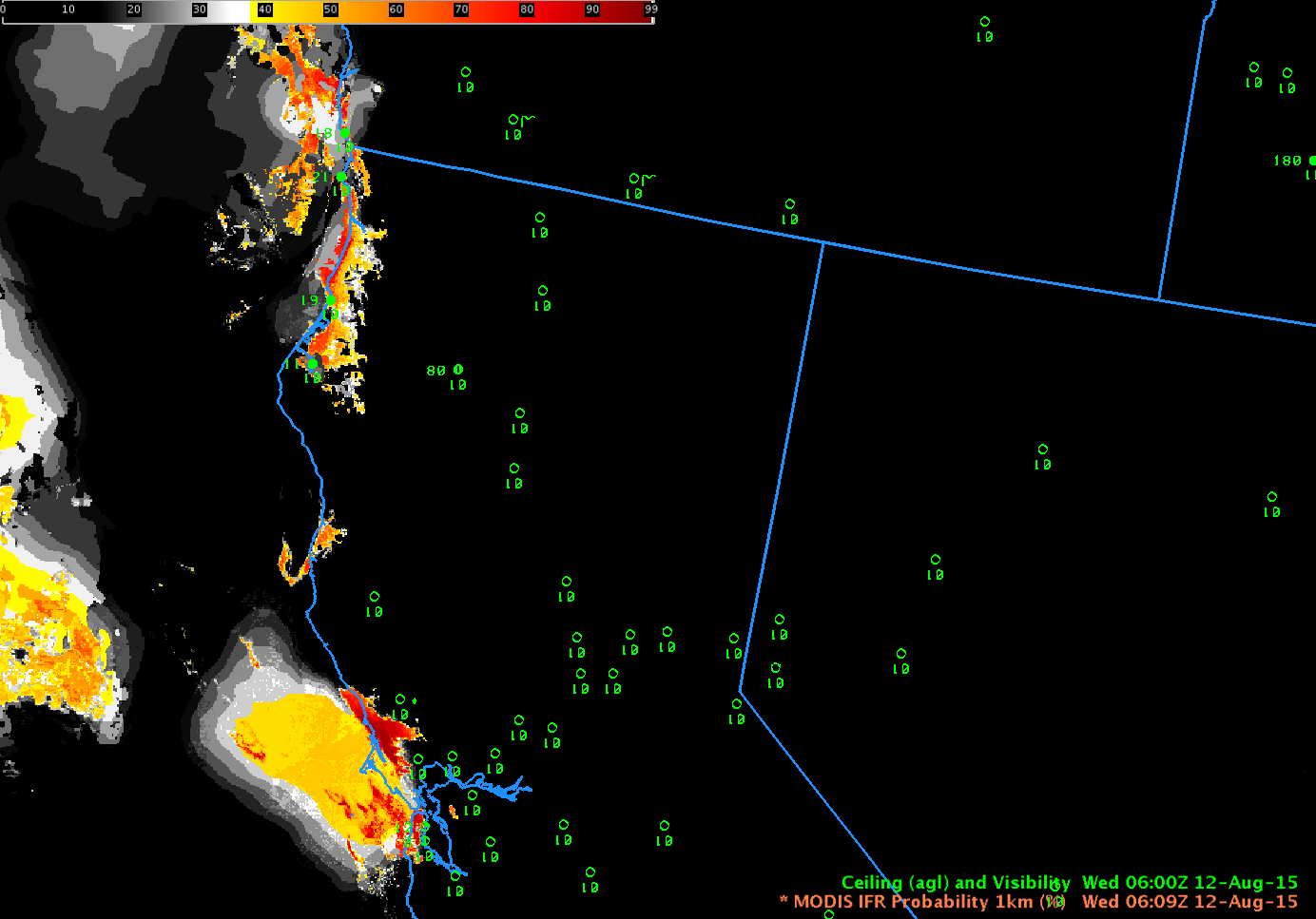
Terra MODIS-based GOES-R IFR Probability fields, 0609 UTC, 12 August 2015 (Click to enlarge)

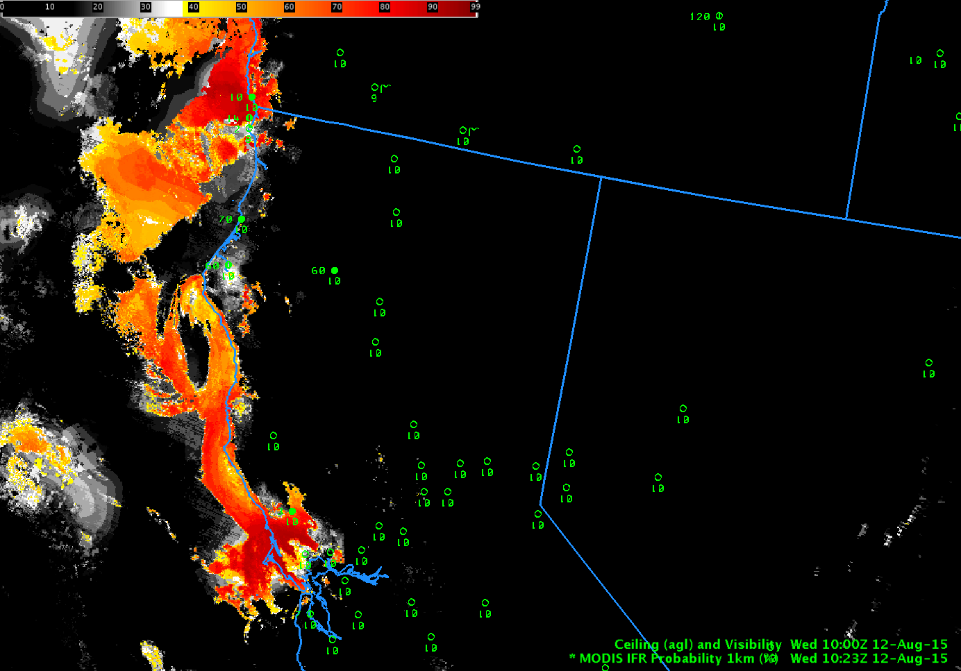
Aqua MODIS-based GOES-R IFR Probability fields, 1023 UTC, 12 August 2015 (Click to enlarge)

MODIS can give high-resolution imagery, but the infrequency of the scenes tempers its usefulness. In contrast, GOES-15 (as GOES-West) views the California coast every 15 minutes, and this excellent temporal resolution (that will improve in the GOES-R era) allows a better monitoring of the evolution of coastal fog. Hourly plots of GOES-R IFR Probability, below, computed from GOES-15 and Rapid Refresh Data show the slow increase in GOES-R IFR Probabilities along the coast as ceilings and visibilities drop.

GOES-R IFR Probability fields, 0400-1200 UTC 12 August 2015 (Click to enlarge)

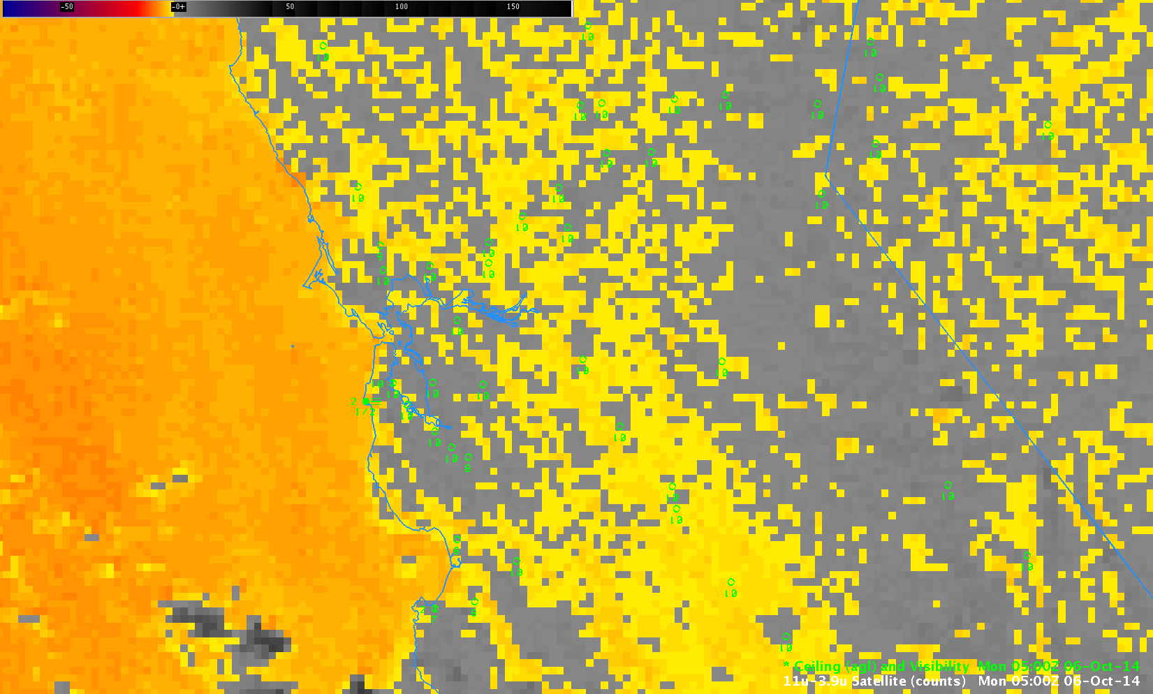
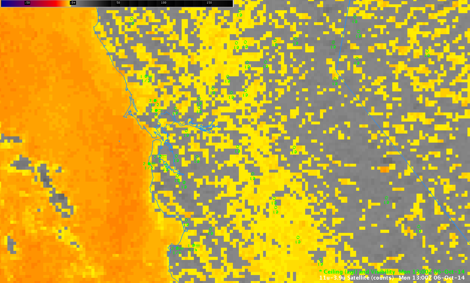
In the animation above, note the general increase in GOES-R IFR probabilities at 0900 UTC relative to 0800 and 1000 UTC. We are close enough to the Solstice that Stray Light Issues are starting. The 0800, 0900 and 1000 UTC brightness temperature difference imagery, below, shows the large signal increase at 0900 UTC that can be attributed to stray light. GOES-R IFR Probabilities can tone down that increase somewhat — because the model data will now show low-level saturation in regions where stray light erroneously suggests low clouds/fog might exist. GOES-R IFR Probabilities also screen out the constant fog signal over the Central Valley of California (and over Nevada) that is driven not by the presence of low clouds but by soil emissivity differences.

GOESWBTD_12August2015_0800_0900_1000step

GOES-15 Brightness Temperature Difference (10.7 µm – 3.9 µm), 0800, 0900 and 1000 UTC 12 August 2015 (Click to enlarge)

======================== Added =========================GOES-14 in SRSO-R mode (see also this link) viewed the west coast starting at 1115 UTC today. The Brightness Temperature Difference field, below, (click here for mp4) shows the slow expansion/evaporation of the low stratus/fog. (GOES-R IFR Probabilities were not computed with the GOES-14 1-minute imagery). The rapid change in the field at sunrise occurs because solar radiation at 3.9 µm quickly changes the brightness temperature difference from negative to positive.

GOES14_BTD_12August2015_1115_1526UTCanim

GOES-14 Brightness Temperature Difference (10.7 µm – 3.9 µm), 1115-1526 UTC 12 August 2015 (Click to view animation)

Visible Imagery is below (Click here for mp4).

960x1280_AGOES14_B1_GOES14_W_animated_2015224_133000_182_2015224_170000_182_GRAY

GOES-14 Visible Imagery (1330-1700 UTC) (Click to animate)

Resolution Matters

GOES-R IFR Probabilities computed from MODIS data and from GOES-15 data, ~1000 UTC on 22 June 2015 (Click to enlarge)

GOES-R IFR Probability was created with an eye towards using data from GOES-R (currently scheduled for launch at the end of March 2016). GOES-R will have better spatial, temporal and spectral resolution than the present GOES. A benefit of better spatial resolution is shown in the toggle above between present GOES (nominal 4-km resolution — vs. the nominal 2-km resolution that will be on GOES-R) and MODIS (1-km resolution). The small valleys along the northern California coastline are far better resolved. The fog/low clouds over San Francisco bay is also better resolved (and the same could be said for the Salinas Valley, south of Monterey Bay if this scene were shifted slightly south). (You might notice a slight 1-pixel shift between MODIS and GOES-15 IFR Probabilities. GOES-15 navigation is compromised by the lack of star-tracking data, so MODIS data are probably better navigated.)

GOES-15 Brightness Temperature Difference (10.7 µm – 3.9 µm) and GOES-R IFR Probabilities, 1000 UTC on 22 June 2015 (Click to enlarge)

IFR Probabilities are derived from GOES-15 brightness temperature difference fields, and a benefit of the IFR Probabilities is obvious above. Brightness Temperature Differences can be driven by emissivity differences in soil. These false positives over Nevada (from the point of view of fog detection) are easily removed if the Model Data does not show low-level saturation.

Suomi NPP Day/Night band imagery, Brightness Temperature Difference Fields (11.45 µm – 3.74 µm), and 3.74 µm Image, 0921 UTC on 22 June 2015 (Click to enlarge)

Suomi/NPP’s early morning overpass also detected the presence of fog/low stratus over the valleys along the northern California coast. The Brightness Temperature Difference field shows things distinctly. The Day-Night Visible imagery shows little in the way of fog on this day, as the waxing crescent moon had already set so no lunar illumination was present. The Day Night band is included here because it shows a very bright wildfire south of Lake Tahoe. That feature is also present in the 3.74 µm imagery. Fog and stratus is also evident in the 3.74 µm imagery, detectable based on its very smooth appearance.

Fog over Coastal California

GOES-R IFR Probabilities computed from GOES-West and Rapid Refresh Data, 0300-1200 UTC on 29 May 2015 (Click to enlarge)

GOES-R IFR Probability fields are challenged most days by the diurnal penetration of coastal fog and stratus that occurs overnight along the California Coast. In the animation above, IFR Probabilities increase in regions along the coast, and also in valleys (such as the Salinas Valley) where fog moves inland. Note above how Monterey, Watsonville and Paso Robles all show IFR (or near-IFR) conditions as the IFR Probabilities increase. The same is true farther north at Santa Rosa and at Marin County Airport, and farther south at Avalon, Ontario, Point Mugu and LA International. IFR Probability fields routinely do capture these common fog events.

The Brightness Temperature Difference Field (10.7 µm – 3.9 µm), below, captures the motion of these low clouds as well. However, numerous ‘false positive’ signals occur over the central Valley of California (likely due to differences in soil emmissivities). The GOES-R IFR Probability field can screen these regions out because the Rapid Refresh data in the region does not show saturation in the lowest kilometer. Note also how the Brightness Temperature Difference field gives little information about low clouds where high clouds are present (over the Pacific Ocean in the images below). IFR Probability fields, however, do maintain a strong signal there because data from the Rapid Refresh strongly suggests the presence of low clouds/fog.

GOES Brightness Temperature Difference Fields, 0400-1200 UTC on 29 May 2015 (Click to enlarge)

Suomi NPP makes an overflight over the West Coast each day around 1000 UTC, and the toggle of the Day Night Band and the Brightness Temperature Difference field (11.45 µm – 3.74 µm) is shown below. The moon at this time was below the horizon, so illumination of any fog is scant; the brightness temperature difference field does highlight regions of water-based clouds (that is, stratus); however, it does not contain information about the cloud base. In other words, it’s difficult to use the brightness temperature difference product alone to predict surface conditions.

1010 UTC Imagery from Suomi NPP VIIRS Instrument: Day Night Visible Band (0.70µm) and Brightness Temperature Difference Field (11.45µm – 3.74µm) (Click to enlarge)

GOES-14 is in SRSO-R mode, and its view today includes the west coast. The animation below shows the erosion of the fog after sunrise at 1-minute intervals. (Click here for mp4, or view it on YouTube). (Click here for an animation centered on San Francisco).

GOES-14 Visible (0.6263 µm) animation, 29 May 2015 [click to play very very large animation]

When Cirrus overlies Fog

GOES-15 Visible Imagery at 1800 UTC on 12-15 January 2015 (Click to enlarge)

Fog and low stratus has persisted in California’s central valley during the week of 12-16 January 2015. The visible imagery above shows the extent of the fog/low stratus at 1800 UTC on 12-15 January.

During the early morning hours of 16 January, high cirrus started to overspread the central Valley (That cirrus is apparent in the visible iamgery from 15 January above). The presence of cirrus makes use of the traditional method of fog detection — brightness temperature difference — problematic because the satellite no longer senses radiation from the low clouds; rather, cirrus radiation is being detected.

The four toggles below show Brightness temperature Difference and GOES-R IFR Probabilities at 0300 (top), 0700 (second from top), 1100 (second from bottom) and 1400 UTC (bottom) on 16 January 2015. At 0300 UTC, cirrus has overspread the northern part of the central Valley. At this time Merced, CA, shows IFR conditions. IFR Probabilities under the cirrus there show a flat field characteristic of conditions when IFR Probabilities are governed by Rapid Refresh data only. Probabilities are higher where satellite data are also included as predictors.

At 0700 UTC and 1100 UTC, cirrus has overspread the entire valley (with occasional breaks). Values of GOES-R IFR Probability are therefore suppressed, so interpretation of the IFR Probability value should be tempered by knowledge of the cloud field. A low value under clear skies means something different than a low value under a cirrus canopy. Under a cirrus canopy, the accuracy of the GOES-R IFR Probability Field depends on the accuracy of the Rapid Refresh model.

AT 1400 UTC, as the cirrus shield retreats, IFR Probabilities increase again over the central Valley.

Toggle between GOES-R IFR Probabilities from GOES-15 and Brightness Temperature Difference Fields, 0300 UTC 16 January 2015 (Click to enlarge)

Toggle between GOES-R IFR Probabilities from GOES-15 and Brightness Temperature Difference Fields, 0700 UTC 16 January 2015 (Click to enlarge)

Toggle between GOES-R IFR Probabilities from GOES-15 and Brightness Temperature Difference Fields, 1100 UTC 16 January 2015 (Click to enlarge)

Toggle between GOES-R IFR Probabilities from GOES-15 and Brightness Temperature Difference Fields, 1400 UTC 16 January 2015 (Click to enlarge)

IFR Probabilities in High Terrain

GOES-15-based GOES-R IFR Probabilities, hourly from 0000 UTC through 1500 UTC on 18 December 2014 (Click to enlarge)

IFR Probabilities give information about IFR Conditions that occur when terrain ascends up into the clouds, as happens sometimes in the Sierras. A stratus deck might exist over the Central Valley of California, but as that stratus extends to the east, the terrain rises up into the cloud, and IFR conditions result. The animation above shows IFR Probabilities during the night of 17-18 December 2014. Stations at elevation are not common, but Blue Canyon (KBLU) in Placer County is at 1600 meters above sea level. IFR Probabilities in/around north central Placer County (where KBLU is sited) are highest with the visibility is most restricted. Note in the animations that Truckee, CA, to the east of Blue Canyon, does not experience IFR Conditions, perhaps because it is east of the crest of the Sierras.

MODIS data occasionally gives very high-resolution information. The data below from 2100 UTC on 17 December and shows the IFR Probability banked up against the Sierras.

MODIS-based GOES-R IFR Probability, 2113 UTC on 17 December 2014, along with surface-based observations of ceilings and visibilities (Click to Enlarge)

Fog near Hanford California

Tweeted Message from the National Weather Service in HNX (Hanford, CA) showing GOES-R IFR Probabilities in the central Valley of California (click to enlarge)

The National Weather Service in Hanford tweeted the image, above, of IFR Probability this morning. How did the evolution of IFR Probabilities compare to that of brightness temperature difference fields?

The hourly animation, below, suggests that data from the Rapid Refresh model was likely crucial in determining exactly where the lowest visibility occurred; the brightness temperature difference field did not capture the horizontal extent of the narrow band of fog that developed to the east of Interstate 5 (The interstate is the purple line in the animation). Indeed, the brightness temperature difference field appears to offer little in the way of forecast value, and differences trend to zero as the sun starts to rise at the end of the animation. In contrast, both IFR and LIFR Probabilities have peak values where ceilings are obscured and visibilities are near zero, in and around Hanford, and those large values persist through sunrise.

Hourly GOES-R IFR Probabilities (Upper Left, computed with data from GOES-15) with ceilings and visibilities plotted, Hourly GOES-R LIFR Probabilities computed with data from GOES-15 (Lower Left), GOES-15 Brightness Temperature Difference (10.7µm – 3.9µm) (Upper Right), Suomi NPP Day Night Band and Brightness Temperature Difference (11.45µm – 3.74µm) (Lower Right), times as indicated (Click to enlarge)

Suomi NPP overflew the central Valley at 0938 UTC. The Day Night Band and the brightness temperature difference (11.45µm – 3.74µm) field, below, do not contain signatures of dense fog near Hanford.

As above, but at 0945 UTC, when Suomi NPP data were present (Click to enlarge)

The two-hour time-lapse video, below, shows the evolution of the Fog at the National Weather Service Office in Hanford on the morning of 4 November.

Successive Suomi NPP Scans Show Stratus/Fog movement

Suomi NPP Day/Night Band at 0926 and 1106 UTC on 9 October 2014 (Click to enlarge)

(A Blog post on Suomi NPP Imagery over the western US from 10 October is available here).

Polar orbiters typically don’t give good temporal resolution, especially near the Equator. In mid-latitudes, however, Polar Geometry can yield views over a wide area on two successive scans. This happened along the West Coast early in the morning on 9 October. Two regions show noticeable changes in stratus between the two times: stratus/fog extends farther down the Salinas Valley at the southern edge of image, and stratus/fog expands over southwestern Puget Sound in Washington. The Brightness Temperature Difference field (11.35µm – 3.74µm) from Suomi NPP for the same times shows a similar evolution over the Salinas Valley, but the view of Washington is obscured by thin cirrus. These cirrus (that show up as black enhancements below) are mostly transparent in the Day Night Band but not in the infrared bands.

Suomi NPP Brightness Temperature Difference (11.35µm – 3.74µm) at 0926 and 1106 UTC on 9 October 2014 (Click to enlarge)

MODIS instruments onboard Terra and Aqua yield spectral data that can be used to generate GOES-R IFR Probability Fields. The animation below shows high-resolution imagery of where IFR Probabilities are highest, but only at three distinct times: 2152 UTC on 8 October and 0537 and 0949 UTC on 9 October. An increase in IFR Probabilities around Monterey Bay is apparent (and consistent with the Suomi NPP Observations above); IFR Probabilities also increase along the Oregon Coast and around Puget Sound.

MODIS-based GOES-R IFR Probabilities at 2152 UTC 8 October, 0547 UTC 9 October and 0949 UTC 9 October (Click to enlarge)

How do GOES-based observations complement the Polar Orbiter data above?

GOES-15 based GOES-R IFR Probabilities, hourly from 0200 through 1400 UTC, 9 October 2014 (Click to enlarge)

The hourly animation above shows the slow increase of IFR Probability in/around Monterey Bay, and also a push of higher IFR Probability onto the Oregon Coast that occurs after the last MODIS-based IFR Image shown farther up. (Higher IFR Probabilities also spill into San Francisco Bay). Do surface observations of ceilings and visibilities agree with the IFR Probability fields? The loops below, from Oregon (below) and Monterey Bay (bottom) suggest that they do. For example, Eugene OR (and stations north and south of Eugene) show IFR conditions as the high IFR Probability field moves in after 1100 UTC. GOES-based data is valuable in monitoring the motion of IFR Probability fields; keep in mind, though, that small-scale features may be lost. For example, it is difficult for GOES to resolve the Salinas Valley.

GOES-15 based GOES-R IFR Probabilities, hourly from 0200 through 1500 UTC, 9 October 2014, with surface and ceiling observations superimposed (Click to enlarge)

GOES-15 based GOES-R IFR Probabilities from 0400 through 1400 UTC, 9 October 2014, with surface and ceiling observations superimposed (Click to enlarge)

IFR Probability along the West Coast

MODIS data from Terra and Aqua, Suomi NPP data, and GOES-15 data yield different types of information that can be used to observe clouds in a region. Probabilities of IFR conditions — that is, what’s going on at cloud base, which is a part of the cloud the satellite cannot see — can be produced by combining satellite observations of cloud tops and data from a model (such as the Rapid Refresh) that includes accurate predictions low-level moisture.

GOES-based IFR Probabilities (Upper Left), GOES-15 Brightness Temperature Difference (10.7µm – 3.9µm) (Upper Right), MODIS-based IFR Probabilities (Lower Right) at 0646 UTC, 0919 and 1058 UTC (Click to enlarge)

The three MODIS images, above (bottom right), show the slow encroachment of higher IFR Probabilities east-southeastward along the Sonoma/Marin county border. The high-resolution imagery from MODIS allows a more accurate depiction of the sharp edges that can occur as marine stratus penetrates inland around topographic features. MODIS data also suggests reduced ceilings in San Francisco.

As above, but at 0919 UTC only, with a toggle of MODIS Brightness Temperature Difference (11µm – 3.7 µm) and IFR Probability (Bottom Right) (Click to enlarge)

The 0919 UTC MODIS pass (from Aqua) happened to pass at a time when the GOES-West brightness temperature difference field was contaminated by stray light. The toggle above shows the difference between MODIS and GOES Brightness Temperature Difference fields at that time. MODIS is only detecting a signal where low clouds are present (or where soil differences allow the emissivitiy differences that can show up in the brightness temperature difference field, in this case over Nevada)

Suomi NPP overflew California at 1000 UTC, and those images are below. The brightness temperature difference field, and the Day Night band show clouds offshore, and city lights in and around San Francisco Bay and Monterey Bay. Regions of stratus have moved inland towards southern Sonoma County, over San Francisco, and over Monterey. There is a slight brightness temperature difference signal in the Suomi NPP data that extends down the Salinas Valley as well; it’s difficult to perceive cloudiness in the Day Night band in that region however.

As above, but with a toggle of Suomi NPP Brightness Temperature Difference and Day Night Band in the lower left, data at 1021 UTC (Click to enlarge)

The great strength of GOES data is its ability to monitor continuously the West Coast. Trends are therefore more easily observed. The hourly loop, below, shows that along much of the west coast, marine stratus stayed off shore through the night. Higher IFR Probabilities are also confined to regions where ceilings and visibilities were reduced. This is an improvement on the brightness temperature difference fields for the same time that have strong signals over much of the central Valley (for example, at 0500 and 1300 UTC, as well as at 0915 UTC, above).

GOES-15 IFR Probabilities, hourly from 0400 through 1300 UTC, 6 October 2014 (Click to enlarge)

MODIS-based IFR Probability over California

MODIS-based IFR Probabilities over the western US, 0932 UTC on 30 June 2014 (Click to enlarge)

MODIS data, although infrequent, can give a high-resolution estimate of whether of not fog/low clouds are forming in a region. This is particularly useful for cases with highly variable terrain (such as deep river valleys). In the image above, IFR Probabilities are very low over both the Central Valley of California and over the Salinas Valley closer to the coast. Fog/low Stratus are unlikely to be occurring.

Suomi/NPP Brightness Temperature Difference Fields (11.35µm – 3.74µm) at 0916 and 1057 UTC on 30 June 2014 (Click to enlarge)

The orbital geometry of Suomi/NPP on June 30th was such that it provided two close-up views of these two valleys around/after the time of the MODIS pass shown above. The animation above toggles between those two times. The brightness temperature difference field shows a general increase in return signal strength. But the MODIS IFR Probability field, top, and GOES-West IFR Probability fields (not shown) support the view that any clouds present are not having an impact on ceilings and visibility. A toggle that includes ceilings and visibilities is here.

Note that returns that suggest low clouds over Nevada are more likely due to emissivity differences in different soils, an effect that is more obvious in very dry conditions.

The Suomi/NPP Day/Night band can also provide imagery to help identify the tops of clouds. However, Day/Night Band imagery uses reflected moonlight. There was a new moon on June 27th, and that almost-new moon had set by the time of the images below. Thus, only Earthglow is illuminating any clouds that are present, and that feeble light is mostly overwhelmed by emitted city lights. It is therefore very difficult to identify any changes in cloudcover from the Day/Night band on this date.

Suomi/NPP Day/Night Band imagery at 0916 and 1057 UTC on 30 June 2014 (Click to enlarge)

GOES-R Fog Product Examples

Fog detection fusing GOES, Terra/Aqua or Suomi/NPP Satellite data with Model output