See the CIMSS Satellite Blog for an analysis of this event from 25 September 2015.
Author Archives: Scott Lindstrom
IFR Probabilities give information during the day too
GOES-R IFR Probabilities, hourly from 1300-1700 UTC on 24 September 2015 (Click to enlarge)
Ceilings and visibilities over South Carolina decreased during the day on 24 September 2015. The animation of hourly IFR Probability fields, above, shows an increase in Probability over South Carolina as the visibilities decreased. IFR Probability fields can alert a forecaster to the possibility of IFR conditions at any time of the day. Visible imagery for the same period, below, shows the multiple cloud layers streaming inland. The accuracy of the IFR Probability field in highlighting the region with near-IFR and IFR Probability is testimony to the accuracy of the Rapid Refresh model data that are used.
GOES-East Visible (0.63 µm) Imagery, hourly from 1300-1700 UTC on 24 September 2015 (Click to enlarge)
IFR Probability vs. Brightness Temperature Difference
GOES-R IFR Probability and GOES-13 Brightness Temperature Difference (10.7 µm – 3.9 µm) at 1000 UTC on 21 September 2015 (Click to enlarge)
The toggle above compares GOES-R IFR Probability fields and GOES-13 Brightness Temperature Difference fields at 1000 UTC on 21 September 2015. A shortcoming of Brightness Temperature Difference fields, or indeed of any low cloud detection algorithm that relies solely on cloud-top measurements, is that low stratus that does not reduce visibility and fog that does reduce visibility can look very similar from the cloud top. By incorporating surface and near-surface moisture information from the Rapid Refresh Model, the GOES-R IFR Probability algorithm can correctly screen out regions of stratus and highlight only those regions where fog and low stratus might affect transporation. In the example above, Guymon OK and Lamar CO are at the outer edge of the highest IFR Probability, and both report IFR conditions. South and west of those stations, IFR Probabilities drop quickly, but brightness temperature difference signals remain strong.
Cloud Thickness and Dissipation Time

Dissipation time as a function of GOES-R Cloud Thickness
The chart above shows the relationship between the last pre-sunrise GOES-R Cloud Thickness product and Fog Dissipation time. Observations of the last pre-sunrise GOES-R Cloud Thickness (developed from an empirical relationship between 3.9 µm emissivity and sodar-observed cloud thickness of the west coast of the USA) can be related to the dissipation time relative to the last observation of Cloud Thickness. The scatterplot was developed using data mostly over the southeastern part of the USA, but also over the Great Plains. However, it does have value in other geographic regions too, as shown below.
GOES-R IFR Probabilities and GOES-R Cloud Thickness, 1100 UTC 16 September 2015 (Click to enlarge)
On 16 September, river fog developed over the Ohio River and its tributaries in Ohio, West Virginia and Pennsylvania. The toggle above shows GOES-R IFR Probability and GOES-R Cloud Thickness fields at 1100 UTC on 16 September. This was the last pre-sunrise GOES-R Cloud Thickness over West Virginia (Indeed, the leading edge of twilight — where GOES-R Cloud Thickness is not computed — is apparent at the extreme eastern edge of the image, from Virginia up into central Pennsylvania). The GOES-R Cloud Thickness fields show largest values — around 800 feet — in/around the Ohio River between West Virginia and Ohio. The chart above suggest rapid dissipation. The best fit line (blue) suggests dissipation in about an hour, although there is considerable spread to the values, from 30 minutes up to almost 2-1/2 hours.
Almost two hours later (1245 UTC), fog is still present in isolated patches near the river, and GOES-R IFR Probability fields are suggesting fog is still present as well. The horizontal extent of the GOES-R IFR Probability field is greatly reduced because visible imagery can be used after sunrise to screen out clear regions (Cloud-clearing in the algorithm is more effective). By 1415 UTC (bottom), three hours after the GOES-R Cloud Thickness imagery above, all fog has evaporated.
GOES-R IFR Probabilities and GOES-13 Visible Imagery (with a low-light enhancement), 1245 UTC 16 September 2015 (Click to enlarge)
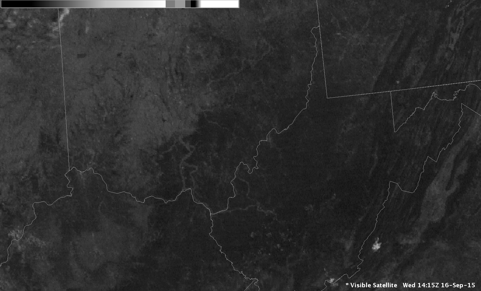
GOES-13 Visible Imagery, 1415 UTC 16 September 2015 (Click to enlarge)
MODIS resolution versus GOES resolution
MODIS-based (0300 UTC) and GOES-based (0315) UTC GOES-R IFR Probability fields on 11 September 2015 (Click to enlarge)
MODIS data (from Terra and Aqua) and GOES data can both be used to create GOES-R IFR Probability fields. The differences between the two data sources — especially spatial resolution — are obvious in the toggle above. MODIS data can capture the development of fingers of fog that develop in small river valleys, and GOES data cannot (although, of course, a forecaster with knowledge of the topography might appropriately tailor a forecast). In the toggle above, MODIS data capture the small tributaries of the Ohio River in Ohio and West Virginia that likely contain fog at 0300 UTC (11 PM local time). GOES data smear out that information. This is true later at night as well, below, at 0715 UTC. River valleys show higher IFR Probabilities than adjacent mountains. Valley fog is easier to delineate with MODIS data than with GOES data.
MODIS-based (0715 UTC) and GOES-based (0715) UTC GOES-R IFR Probability fields on 11 September 2015 (Click to enlarge)
GOES-R IFR Probabilities at High Latitudes
Screenshot from the Juneau, AK WFO on 8 September 2015. The yellow region has a Dense Fog Advisory (Click to enlarge)
A challenge in using GOES-R IFR Probabilities at high latitudes is that GOES pixels are larger, typically twice or three times the size of pixels over the lower 48. If Fog is starting out as a small-scale phenomenon, the early development of the feature can be missed. Dense fog developed over southeast Alaska on the morning of 8 September. The animation of GOES-15-based IFR Probabilities, below, shows the slow increase in areal extent to the IFR Probabilities in the six hours between 0445 and 1045 UTC; values also increased. This slow increase in concert with observations can increase confidence that wide-spread dense fog is possible.
GOES-15 based GOES-R IFR Probabilities, 0445, 0715 and 1045 UTC on 8 September 2015 (Click to enlarge)
MODIS data from Terra and Aqua can also be used to compute IFR Probabilities, and the high resolution information from these two polar orbiting satellites can clarify where fog might be occurring. Additionally, MODIS fields are a bit more frequent over Alaska than they are over the lower 48. The 0600 and 0737 UTC passes, shown below, show how MODIS data can be used to refine the GOES-based information at times during the night. The temporal change between MODIS information at 0600 and 0737 UTC also confirms the trend observed in GOES data alone.
GOES-15 and MODIS-based GOES-R IFR Probabilities, 0600 UTC 8 September 2015 (Click to enlarge)
GOES-15 and MODIS-based GOES-R IFR Probabilities, ~0730 UTC 8 September 2015 (Click to enlarge)
Dense Fog over Kansas

Screen Captures of NWS Pages at Dodge City (left) and Wichita (Right), 0700 CST 31 August 2015 (click to enlarge)
Dense Fog Advisories were issued by both Dodge City and Wichita WFOs on the morning of 31 August 2015. GOES-R IFR Probabilities in this case did a better job of outlining where IFR conditions were occurring, distinguishing those regions from regions of low stratus. Each of the paired images below shows Brightness Temperature Difference fields on top and IFR Probability fields on bottom, for four different times during the night (0530, 0715, 0915, 1115 UTC). IFR Probability fields show a signal that is confined mostly to regions where IFR conditions are developing (for the earlier times) or observed (at 0915 and 1115 UTC). Thus, IFR Probability in this case refines the brightness temperature difference signal, highlighting regions only where low clouds/fog are present (eastern Kansas), rather than regions where stratus clouds are present (western Kansas). The incorporation of near-surface saturation as predicted in the Rapid Refresh model is key to screening out regions of mid-level stratus when low stratus and fog are the more important field.
GOES-13 Brightness Temperature Difference (10.7µm – 3.9µm) (top) and GOES-R IFR Probabilities (bottom), 0530 UTC 31 August 2015 (Click to enlarge)
GOES-13 Brightness Temperature Difference (10.7µm – 3.9µm) (top) and GOES-R IFR Probabilities (bottom), 0715 UTC 31 August 2015 (Click to enlarge)
GOES-13 Brightness Temperature Difference (10.7µm – 3.9µm) (top) and GOES-R IFR Probabilities (bottom), 0915 UTC 31 August 2015 (Click to enlarge)
GOES-13 Brightness Temperature Difference (10.7µm – 3.9µm) (top) and GOES-R IFR Probabilities (bottom), 1115 UTC 31 August 2015 (Click to enlarge)
When the sun rises, solar radiation with a wavelength of 3.9 µm will alter the brightness temperature difference field. At night, a water-based cloud will not emit 3.9 µm radiation as a blackbody and be perceived as colder (compared to 10.7 µm). During the day, the relatively large amount of 3.9 µm radiation from the sun reflected off the cloud will make the cloud appear to be warmer (compared to 10.7 µm). Thus the signal in the brightness temperature difference field flips. In contrast, the IFR Probability field signal is not significantly perturbed by sunrise. The 1315 UTC image, below, is an example of this. The GOES-R IFR probability field also benefits from better cloud clearing during the day.

GOES-13 Brightness Temperature Difference (10.7µm – 3.9µm) (top) and GOES-R IFR Probabilities (bottom), 1315 UTC 31 August 2015 (Click to enlarge)
IFR Probability and fog over the Southeast United States
This blog post shows how IFR Probability fields can give an early alert to the development of IFR Conditions.
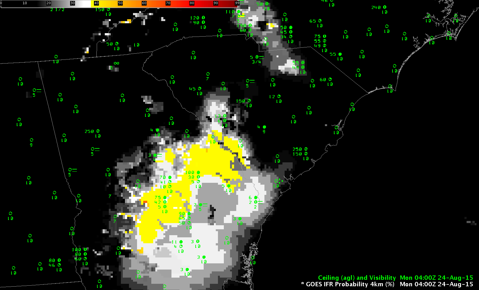
GOES-R IFR Probability fields, 0400 UTC 24 August 2015 (Click to enlarge)
GOES-R IFR Probability fields from 0400 UTC on 24 August 2015, above, show enhanced probabilities over interior southeast Georgia. Observations of surface visibilities and ceilings do not show widespread IFR conditions. But the presence of enhanced values in IFR Probability suggest careful attention should be paid to this region.

GOES-R IFR Probability fields, 0700 UTC 24 August 2015 (Click to enlarge)
Three hours later (0700 UTC), IFR Probabilities have increased somewhat, and some observations are closer to IFR conditions. This is consistent with the slow development of radiation fog overnight over the southeast part of the country.
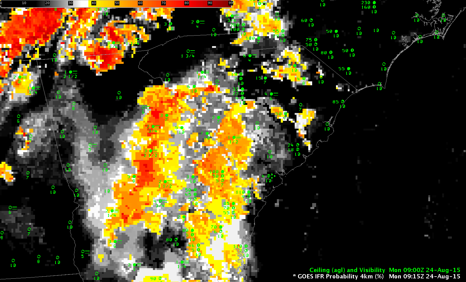
GOES-R IFR Probability fields, 0915 UTC 24 August 2015 (Click to enlarge)
By 0915 UTC, above, IFR Conditions are observed in regions where IFR Probabilities continue to increase. The increase in IFR Probability values continues at 1100 UTC, below, with numerous regions with values exceeding 90%. IFR Conditions are widespread over southeast Georgia and parts of adjacent South Carolina.
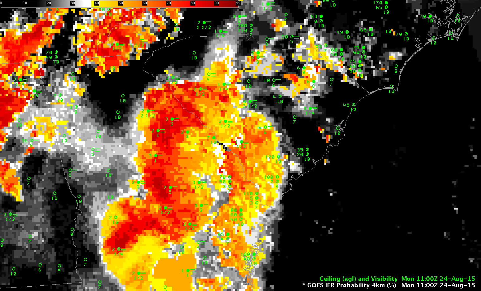
GOES-R IFR Probability fields, 1100 UTC on 24 August 2015 (Click to enlarge)

IFR Probability fields are consistent through sunrise, with values exceeding 90% after the sun has risen, at 1300 UTC, above. The cloud-clearing that can be done with visible imagery at 1300 UTC means the edges of the fog field are more sharply defined at 1300 UTC than they were at 1100 UTC.
Dense Fog over central Nebraska
GOES-R IFR Probability (Upper Left), GOES-R Low IFR Probability (Lower Left), GOES-13 Brightness Temperature Difference Field (10.7 µm – 3.9 µm) (Upper Right), GOES-R Cloud Thickness (Lower Right), Times as Indicated (Click to enlarge)
GOES-R IFR Probability fields, above, suggest IFR conditions are developing over central Nebraska during the early morning of 18 August 2015. Several aspects of the field require comment. At the beginning of the animation, there are noticeable north-south oriented lines in the IFR and Low-IFR Probability fields. These are artifacts of determining the saturation in the lowest 1000 feet of the model as discussed here. As the model saturation deepened over the course of the night, those parallel lines disappeared.
The flat nature of the field announces that satellite data are not being used in the computation of IFR Probability because multiple cloud layers are present. Model fields lack the fine spatial resolution of GOES Satellite data. Where breaks in the clouds do occur, GOES-R IFR Probability fields increase in value (because cloud predictors can be used, and their use enhances the ability of the algorithm to predict whether fog/low clouds are present): Temper your interpretation of the magnitude of the IFR Probability with knowledge of presence of clouds.
Note that the Brightness Temperature Difference field at 0500 UTC has much larger values. Stray Light is beginning to impinge on satellite fields as the calendar gets closer to the Equinox. This issue will remain through mid-October. Multiple cloud decks over Nebraska on 18 August greatly hampered the ability of the brightness temperature difference field to identify regions of low clouds.
The GOES-R Cloud Thickness fields are displayed; these are derived from an empirical relationship between 3.9 µm emmissivity and cloud thickness derived from SODAR data off the west coast of the United States. When multiple cloud layers are present, this field is not computed (nor is it displayed around sunrise/sunset). Thus, you should not see Cloud Thickness fields in regions where GOES-R IFR Probability fields are very smooth (suggesting that only model data are being used). The regions where Cloud Thickness is displayed, above, correspond to regions in the IFR Probability field that are pixelated (that is, where satellite data are being used).
Fog formation is aided by increasingly long nights. Nights now are above 90 minutes longer in Hastings than they were at the Summer Solstice.
The text for the advisory is below:
URGENT - WEATHER MESSAGE
NATIONAL WEATHER SERVICE HASTINGS NE
608 AM CDT TUE AUG 18 2015

...DENSE FOG PERSISTING FOR A FEW HOURS THIS MORNING...

NEZ048-049-061>064-073>077-181400-
/O.NEW.KGID.FG.Y.0006.150818T1108Z-150818T1400Z/
MERRICK-POLK-BUFFALO-HALL-HAMILTON-YORK-PHELPS-KEARNEY-ADAMS-CLAY-
FILLMORE-
INCLUDING THE CITIES OF...CENTRAL CITY...STROMSBURG...OSCEOLA...
SHELBY...POLK...KEARNEY...GRAND ISLAND...AURORA...YORK...
HOLDREGE...MINDEN...HASTINGS...SUTTON...HARVARD...CLAY CENTER...
EDGAR...FAIRFIELD...GENEVA...EXETER...FAIRMONT
608 AM CDT TUE AUG 18 2015

...DENSE FOG ADVISORY IN EFFECT UNTIL 9 AM CDT THIS MORNING...

THE NATIONAL WEATHER SERVICE IN HASTINGS HAS ISSUED A DENSE FOG
ADVISORY...WHICH IS IN EFFECT UNTIL 9 AM CDT THIS MORNING.

* VISIBILITY...REDUCED TO 1/4 MILE OR LESS ACROSS MUCH OF THE
  ADVISORY AREA...INCLUDING THE INTERSTATE 80 AND HIGHWAY 6
  CORRIDORS. THE COMBINATION OF RAIN MOVING INTO PARTS OF THE
  AREA...ALONG WITH A COLD FRONT MOVING IN FROM THE WEST...SHOULD
  HELP TO GRADUALLY IMPROVE DENSE FOG ISSUES.

* IMPACTS...DENSE FOG WILL GREATLY AFFECT THE MORNING COMMUTE IN
  SOME AREAS...AND MOTORISTS ARE URGED TO DRIVE WITH CAUTION AND
  PREPARE FOR RAPID CHANGES IN VISIBILITY OVER SHORT DISTANCES.

PRECAUTIONARY/PREPAREDNESS ACTIONS...

A DENSE FOG ADVISORY MEANS VISIBILITIES WILL FREQUENTLY BE
REDUCED TO LESS THAN ONE QUARTER MILE. IF DRIVING...SLOW DOWN...
USE YOUR HEADLIGHTS...AND LEAVE PLENTY OF DISTANCE AHEAD OF YOU.

&&

$$

PFANNKUCH
Coastal California Fog
Toggle between Suomi NPP Day Night Band Visible (0.70 µm) Image and Brightness Temperature Difference (11.45 µm – 3.74 µm) , 1003 UTC 12 August 2015 (Click to enlarge)
Suomi NPP data from 1003 UTC on 12 August, above, shows evidence of a cloud bank hugging the northern California coast from Cape Mendocino to San Francisco Bay. It also penetrates inland to Santa Rosa in Sonoma County. (Note also how the fires burning in interior show up well in the Day Night Band — they are emitting visible light — and in the Brightness Temperature Difference band — because they are much warmer in the 3.74 µm image than in the 11.45 µm image).
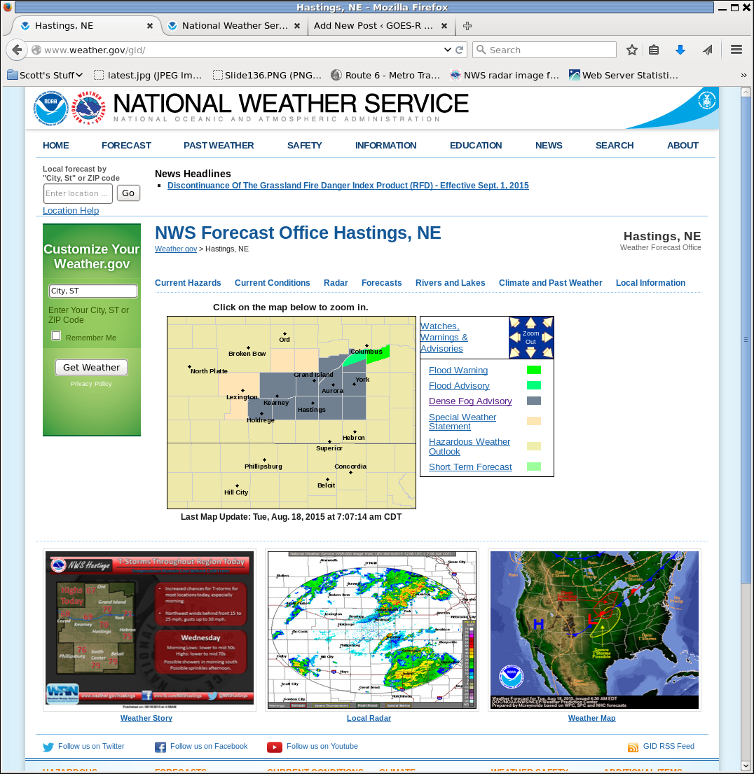
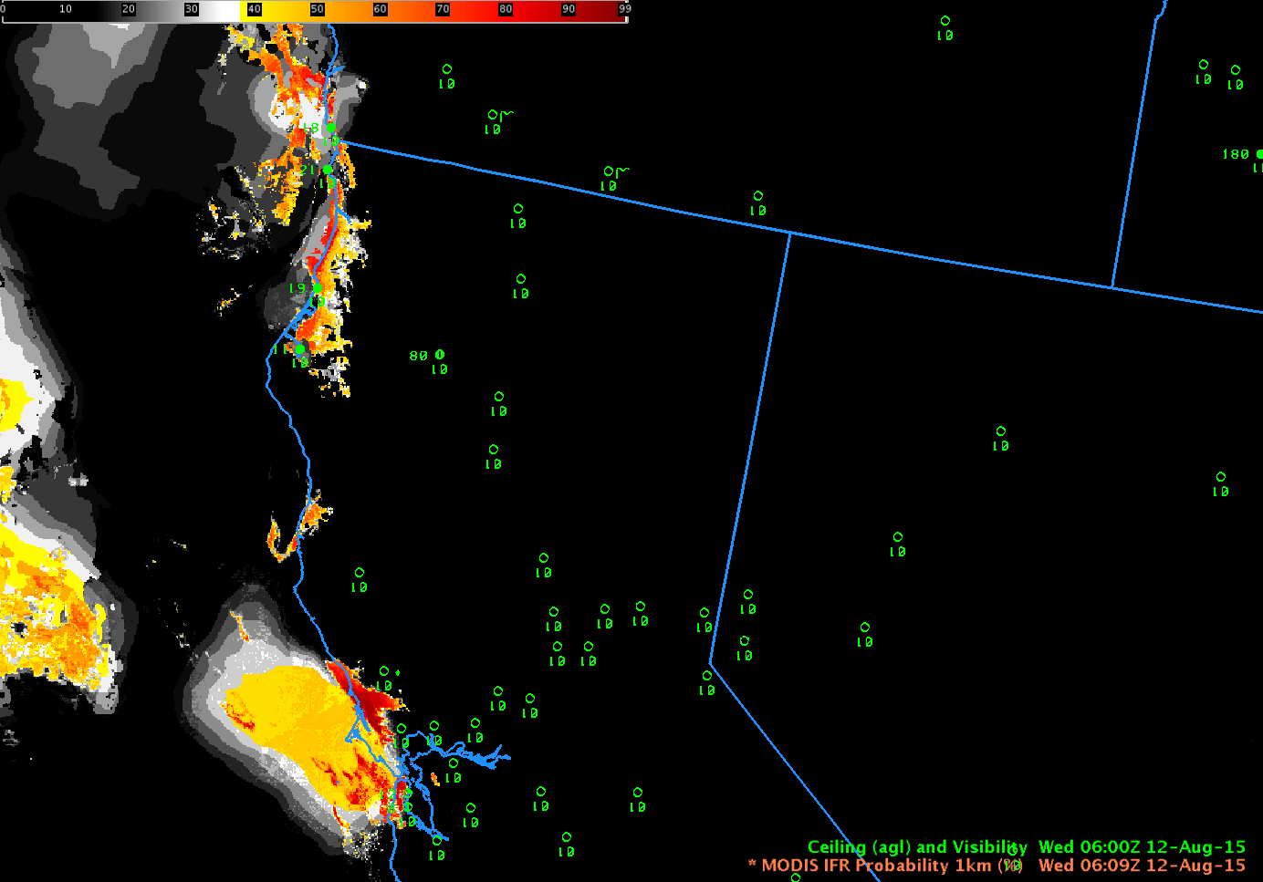
Terra overflew the California coast at ~0600 UTC and Aqua overflew the coast at ~1000 UTC; MODIS-based IFR Probabilities could be constructed from these overpasses, and they are shown below. At 0609 UTC, High IFR Probabilities (>90%) are confined to coastal Sonoma County and along the coast from Humboldt county north. By 1023 UTC, high IFR Probabilities stretch along the entire coast from Cape Mendocino to the mouth of San Francisco Bay, with evidence of inland penetration along river valleys. (The Russian River, for example, and perhaps the Noyo River in Mendocino County)
Terra MODIS-based GOES-R IFR Probability fields, 0609 UTC, 12 August 2015 (Click to enlarge)
Aqua MODIS-based GOES-R IFR Probability fields, 1023 UTC, 12 August 2015 (Click to enlarge)
MODIS can give high-resolution imagery, but the infrequency of the scenes tempers its usefulness. In contrast, GOES-15 (as GOES-West) views the California coast every 15 minutes, and this excellent temporal resolution (that will improve in the GOES-R era) allows a better monitoring of the evolution of coastal fog. Hourly plots of GOES-R IFR Probability, below, computed from GOES-15 and Rapid Refresh Data show the slow increase in GOES-R IFR Probabilities along the coast as ceilings and visibilities drop.
GOES-R IFR Probability fields, 0400-1200 UTC 12 August 2015 (Click to enlarge)
In the animation above, note the general increase in GOES-R IFR probabilities at 0900 UTC relative to 0800 and 1000 UTC. We are close enough to the Solstice that Stray Light Issues are starting. The 0800, 0900 and 1000 UTC brightness temperature difference imagery, below, shows the large signal increase at 0900 UTC that can be attributed to stray light. GOES-R IFR Probabilities can tone down that increase somewhat — because the model data will now show low-level saturation in regions where stray light erroneously suggests low clouds/fog might exist. GOES-R IFR Probabilities also screen out the constant fog signal over the Central Valley of California (and over Nevada) that is driven not by the presence of low clouds but by soil emissivity differences.

GOES-15 Brightness Temperature Difference (10.7 µm – 3.9 µm), 0800, 0900 and 1000 UTC 12 August 2015 (Click to enlarge)
======================== Added =========================
GOES-14 Brightness Temperature Difference (10.7 µm – 3.9 µm), 1115-1526 UTC 12 August 2015 (Click to view animation)
Visible Imagery is below (Click here for mp4).
GOES-14 Visible Imagery (1330-1700 UTC) (Click to animate)