The video below is a short (11-minute) description of IFR Probability.
Alternatively, click the Link.
The video below is a short (11-minute) description of IFR Probability.
Alternatively, click the Link.
Dense Fog advisories were issued by the National Weather Service in Grand Forks as visibilities in the WFO dropped to near zero. How did the IFR Probability Fields and traditional Brightness Temperature Difference Fields capture this event? The animation below shows the brightness temperature difference field (10.7 µm – 3.9 µm) from GOES-13. Initially, a swath of mid-level and upper-level clouds covered the Red River Valley (this system had produced very light rains on Monday the 27th), but the clouds moved east and dense fog quickly developed (Cavalier, ND, for example, showed reduced visibility already at 0400 UTC).
GOES-13 Brightness Temperature Difference (10.7 µm – 3.9 µm) hourly from 0315 to 1115 UTC on 28 April 2015, along with surface plots of ceilings and visibility (Click to enlarge)
The IFR Probability fields for the same time, below, better capture the horizontal extent of the fog. For example, the strong signal in the Brightness Temperature Difference field over South Dakota at the end of the animation, above, is not present in the IFR Probability fields. IFR Conditions are not occurring over South Dakota. The good match between the developing IFR Probability fields and the developing fog testifies to the satellite view of the fog and the accurate simulation of this event by the Rapid Refresh model.
GOES-R IFR Probability Fields hourly from 0315 to 1115 UTC on 28 April 2015, along with surface plots of ceilings and visibility (Click to enlarge)
Geostationary GOES fields give good temporal resolution to the evolving field. Polar orbiting satellites, such as Suomi NPP (carrying the VIIRS instrument) and Terra/Aqua (each carrying MODIS) each gave snapshot views of the developing fog. At 0355, IFR Probabilities are low, and the Red River valley is mostly obscured by higher clouds. Four hours later, at 0805 UTC, dense fog has developed and IFR probabilities are large.
Terra MODIS Brightness Temperature Difference (11µm – 3.9µm) and IFR Probability fields, ~0355 UTC on 28 April 2015 (Click to enlarge)
Aqua MODIS Brightness Temperature Difference (11µm – 3.9µm) and IFR Probability fields, ~0805 UTC on 28 April 2015 (Click to enlarge)
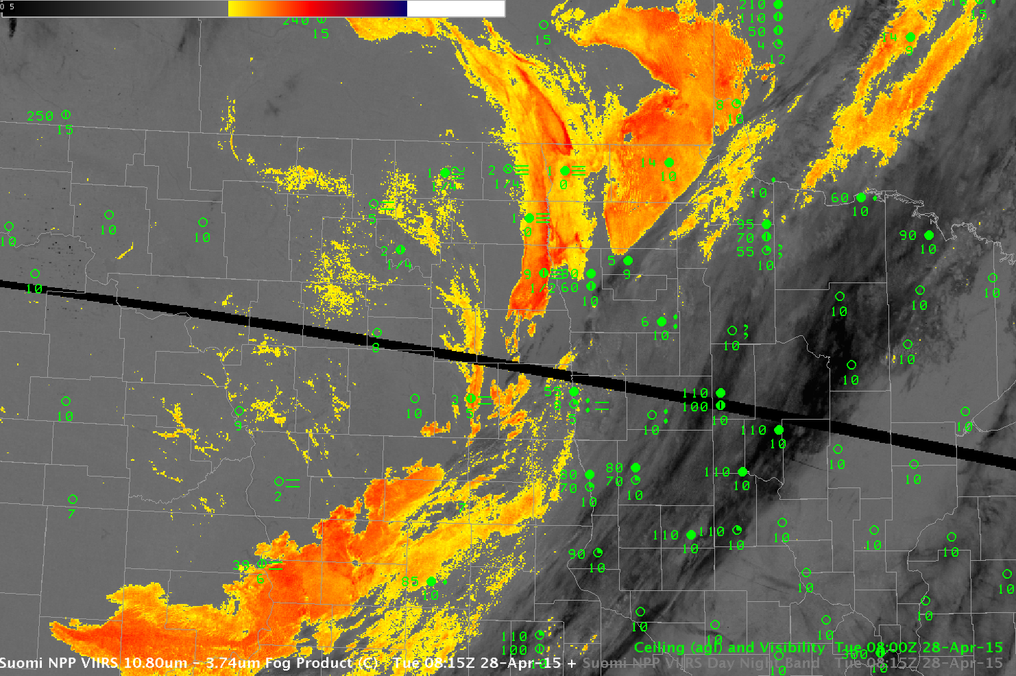
Suomi NPP also viewed the fog field. The toggle between the Day Night Band and the Brightness Temperature Difference field (11.45µm – 3.74µm), below, shows evidence of fog in the visible Day Night band imagery. The lights of western North Dakota’s oil shale fields are also evident.
Polar-orbiting satellites give excellent high-resolution imagery of fog fields. When used in concert with the excellent time resolution of GOES imagery, a complete picture of the evolving fog field can be drawn.
Toggle between Day Night Band (0.70 µm) and Brightness Temperature Difference (11.45µm – 3.74µm) field from VIIRS on Suomi NPP at 0815 UTC (Click to enlarge)
GOES-R IFR Probabilities, 0800 through 1400 UTC on 27 April 2015 (Click to enlarge)
Fog developed along Lake Erie after sunrise on Monday 27 April 2015. The fog and low ceilings were associated with a line of light showers, so multiple cloud layers were present. These layers inhibit satellite detection of fog/low stratus. GOES-R IFR Probabilities, above, computed using GOES-13 Satellite data and Rapid Refresh Model Output show very low probabilities at 0800 and 1015 UTC (stratus clouds are observed); at 1215 UTC, IFR Probabilities increase in the counties adjacent to Lake Erie in Pennsylvania and New York; at 1315 and 1400 UTC, IFR Probabilities are high, and IFR conditions are observed in both Erie PA and Dunkirk NY.
GOES-13 Brightness Temperature Difference Fields, 0400 through 1000 UTC on 27 April 2015 (Click to enlarge)
Brightness Temperature Difference fields overnight, above, showed evidence of water-based clouds over much of the area. The fields are moving south, however, leaving the lakeshore behind. The toggle below is of Brightness Temperature Difference and IFR Probability from 1215 UTC. It is far more difficult to relate features in the brightness temperature difference field with reductions in observations at the surface than it is to relate IFR Probability fields with surface observations. Note also that the character of the brightness temperature difference field below has changed because reflected solar radiation at 3.9 µm has become important.
Toggle between GOES-R IFR Probability fields and GOES East Brightness Temperature Difference Fields at 1215 UTC on 27 April 2015 (Click to enlarge)
GOES-R IFR Probabilities over Indiana and surrounding states, 0200-1215 UTC on 17 April (Click to enlarge)
For developed over Indiana and surrounding states during the morning of April 17th. An hourly animation of GOES-R IFR Probabilities, from 0200 through 1215 UTC, computed from GOES-East and Rapid Refresh Data is shown above. Fog is developing at 0200 UTC, already over portions of western Indiana, and IFR Probabilities increase quickly. By 0700 UTC, large regions show reduced visibilities and IFR Probabilities exceeding 85%.
High clouds moving in from the west and southwest starting at about 0800 UTC have an impact on the IFR Probability fields as well. Only Rapid Refresh Data are used to compute IFR Probabilities where mid-level and high clouds prevent satellite detection of low clouds. As a result, the character of the field changes: it becomes flatter (less pixelated) and values decrease (because probability is not so certain when satellite data cannot be used to validate Model predictions).
The final image in the animation above, at 1215 UTC, was computed just after sunrise. Note that IFR Probability values generally increase. This is especially notable in regions where mid-level and high-level clouds are present (over southern Illinois and southern Indiana). Probabilities are higher because the satellite can detect clouds are present. There are also regions at 1215 UTC where IFR Probabilities rapidly drops to zero. This is likely a difficulty in the Cloud Typing algorithm that occurs with very low sun angle (as discussed here). Holes at 1215 UTC have filled in by 1300 UTC.
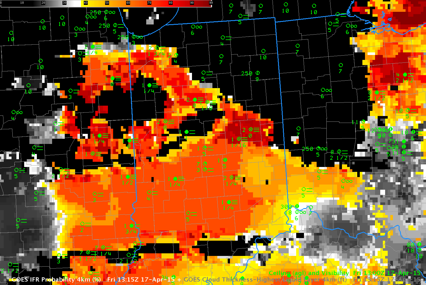
Cloud thickness can give a first estimate of cloud dissipation time. This link shows a scatterplot with a best-fit line that relates dissipation time to Cloud Thickness from a past study. The Cloud Thickness used is the final one computed before twilight conditions, and that is shown below. (Note that cloud thickness is not computed in regions where mid-level and high-level clouds exist) Much of the fog over Indiana is relatively thin — less than 800 feet thick — with a few regions that exceed 1000 feet. Burn-off of this fog should be relatively quick, and most of the Dense Fog Advisories expired at 1400 UTC.
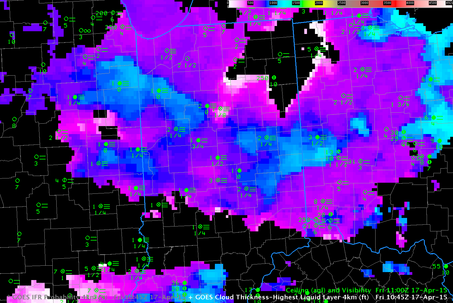
GOES-R Cloud Thickness just before sunrise, 17 April 2015 (Click to enlarge)
URGENT - WEATHER MESSAGE
NATIONAL WEATHER SERVICE NORTHERN INDIANA
600 AM EDT FRI APR 17 2015

INZ020-022-023-032>034-171400-
/O.NEW.KIWX.FG.Y.0005.150417T1000Z-150417T1400Z/
WHITE-CASS IN-MIAMI-GRANT-BLACKFORD-JAY-
INCLUDING THE CITIES OF...MONTICELLO...BROOKSTON...MONON...
LOGANSPORT...ROYAL CENTER...PERU...GRISSOM AFB...MEXICO...
MARION...GAS CITY...UPLAND...HARTFORD CITY...MONTPELIER...
PORTLAND...DUNKIRK
600 AM EDT FRI APR 17 2015

...DENSE FOG ADVISORY IN EFFECT UNTIL 10 AM EDT THIS MORNING...

THE NATIONAL WEATHER SERVICE IN NORTHERN INDIANA HAS ISSUED A
DENSE FOG ADVISORY...WHICH IS IN EFFECT UNTIL 10 AM EDT THIS
MORNING.

* VISIBILITY: A QUARTER MILE OR LESS.

* IMPACTS: VERY HAZARDOUS DRIVING CONDITIONS...WHICH WILL LEAD TO
  TRAVEL DELAYS. PLEASE LEAVE EARLY IF TRAVELING THIS MORNING AND
  ALLOW EXTRA TIME TO REACH YOUR DESTINATION.

PRECAUTIONARY/PREPAREDNESS ACTIONS...

A DENSE FOG ADVISORY MEANS VISIBILITIES WILL FREQUENTLY BE
REDUCED TO LESS THAN ONE QUARTER MILE. IF DRIVING...SLOW DOWN...
USE YOUR HEADLIGHTS...AND LEAVE PLENTY OF DISTANCE AHEAD OF YOU.
GOES-R IFR Probabilities computed from MODIS and from GOES-15, both at ~0700 UTC on 14 April 2015 (Click to enlarge)
At very high latitudes, limb effects can alter the brightness temperature difference between 10.7 µm and 3.9 µm. GOES also has very large pixel sizes at high latitudes. The image above toggles between the GOES-R IFR Probability computed using MODIS and GOES-15. Observations — scant over Alaska — of ceilings and observations are superimposed on the imagery. GOES-based GOES-R IFR Probabilities are elevated over much of Alaska; in contrast, MODIS-based IFR Probabilities show larger values in only a few regions.
MODIS-based values at high latitudes are available frequently compared to lower latitudes. At 0830/0845 UTC, below, MODIS data show a slow expansion in values (note that eastern Alaska was not viewed by MODIS at this time). At about 1100 UTC, the slow areal increase in IFR Probabilities continues.
GOES-R IFR Probabilities computed from MODIS and from GOES-15, both at ~0830 UTC on 14 April 2015 (Click to enlarge)
GOES-R IFR Probabilities computed from MODIS and from GOES-15, both at ~1100 UTC on 14 April 2015 (Click to enlarge)
The 1100 UTC MODIS pass was over only eastern Alaska, and it shows relatively large values in some spots of northeastern Alaska. The high values from the GOES-based GOES-R IFR Probabilities over central Alaska can probably be discounted. Note, however, that the highest GOES-based GOES-R IFR Probabilities do have a counterpart in the MODIS-based field.
At 1400 UTC, no MODIS pass was available. The GOES-based image, below, again has large values over northern Alaska (with corroborating surface observations at Point Lay (where snow is falling) and at Atqasuk (where freezing fog is reported). MODIS-based data from earlier in the day adds confidence to the discounting of widespread modest (40-50%) IFR Probability values over central Alaska.

GOES-R IFR Probabilities computed from GOES-15 at 1400 UTC on 14 April 2015 (Click to enlarge)
GOES-R IFR Probabilities, hourly from 0200 through 1300 UTC on 7 April 2015 (Click to enlarge)
Denver International Airport had a period of restricted visibility during the morning of 7 April, starting around 0830 UTC, when northeast winds ushered in low ceilings and reduced visibilities. High Probabilities in the IFR Probability fields shift west and south with time, demonstrating how the fields can be used to anticipate the development of IFR conditions.
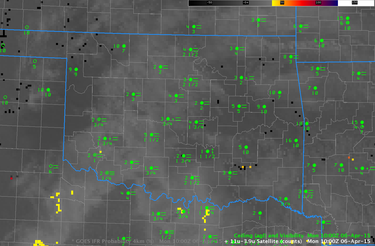
Brightness temperature Difference field (10.7µm – 3.9µm) from GOES East over the southern Plains, 1000 UTC on 6 April 2015 (Click to enlarge)
The heritage, traditional method for detecting fog and low stratus is the brightness temperature difference product, seen above (with an enhancement) at 1000 UTC on 6 April. It is difficult to discern a difference in the field over regions where IFR conditions are reported versus regions where IFR conditions are absent. In contrast, the IFR Probability Field from the same time, below, neatly outlines the regions of IFR conditions, and, importantly, does not highlight regions — such as Fort Smith AR and Poteau, OK — where IFR conditions are not present.
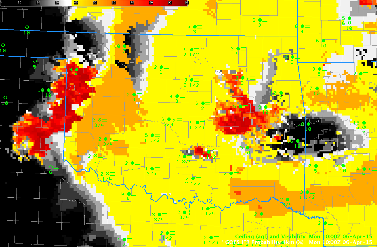
GOES-R IFR Probability Fields, 1000 UTC on 6 April 2015 UTC (Click to enlarge)
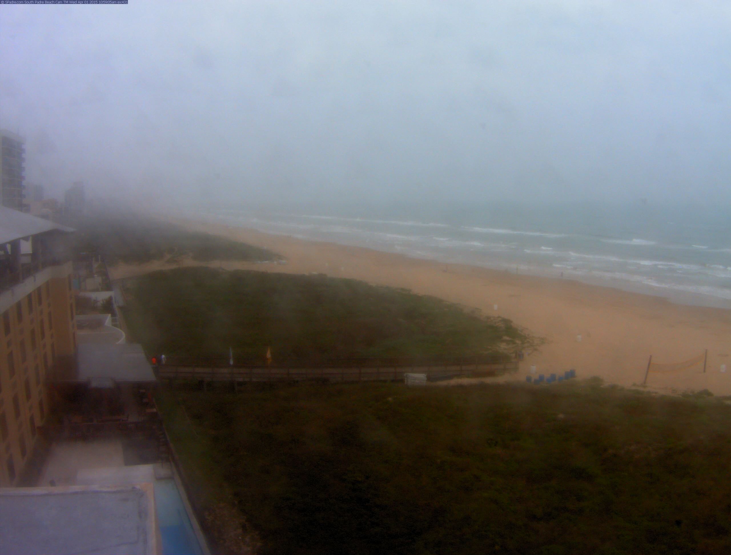
Webcam image of South Padre Island, TX, 11 AM 1 April 2015 (click to enlarge)
Webcam imagery from South Padre Island between 10 and 11 AM on 1 April (above, from this site) showed dense fog that had rolled in from the sea. This is likely an advection fog formed as humid air over the Gulf of Mexico moved over relatively cooler shelf water. SSTs in the region were in the upper 60s (Fahrenheit) as depicted by the image below.
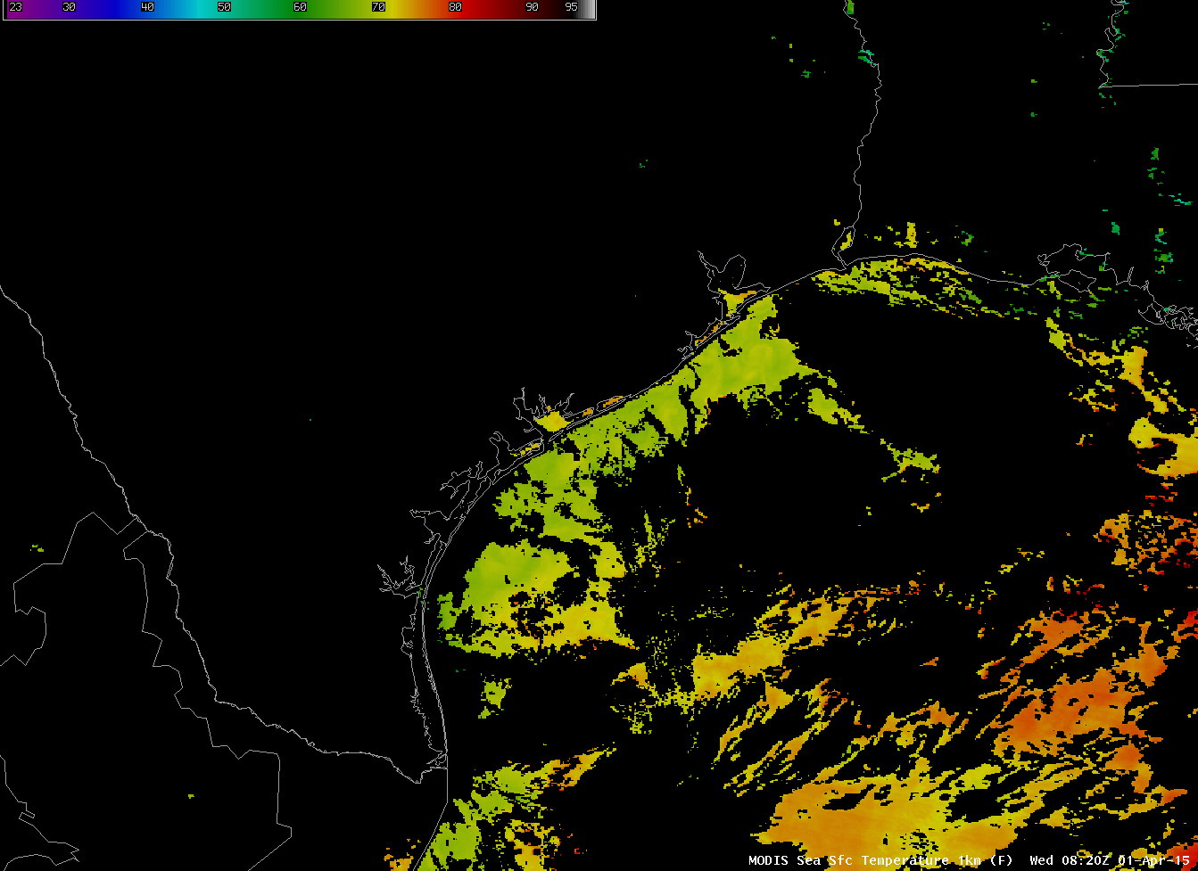
Sea-surface Temperatures, early morning 1 April 2015 (Click to enlarge)
GOES-R IFR Probabilities, below, suggested the presence of the IFR conditions that existed at the coast. Very high probabilities are concentrated near South Padre Island, and spread north and northeastward, with highest values hugging the shoreline.
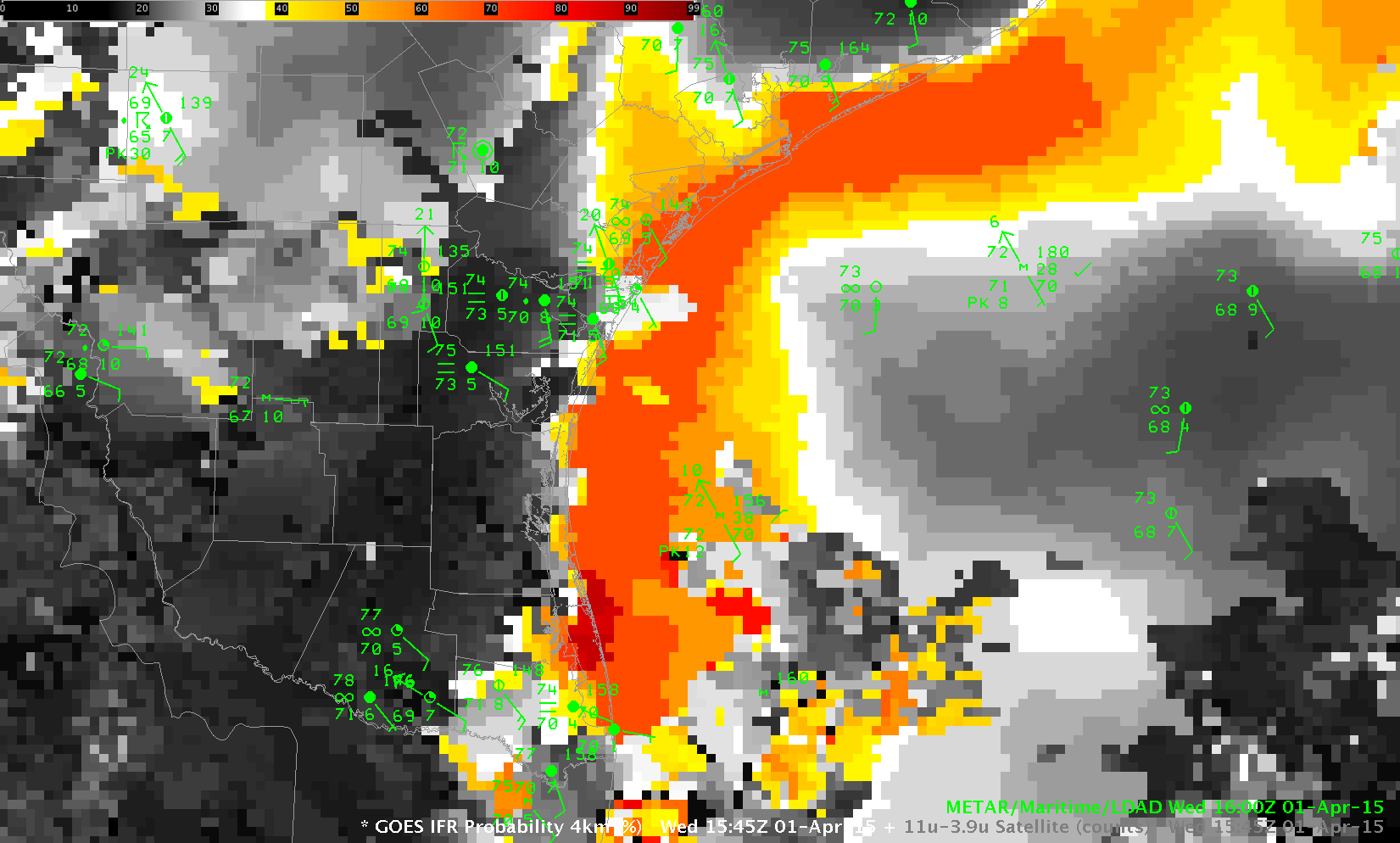
GOES-R IFR Probabilities computed from GOES-East and Rapid Refresh Data, 1545 UTC on 1 April 2015 (Click to enlarge)
Brightness Temperature Difference fields at the same time gave little surface information because of the presence of high clouds.
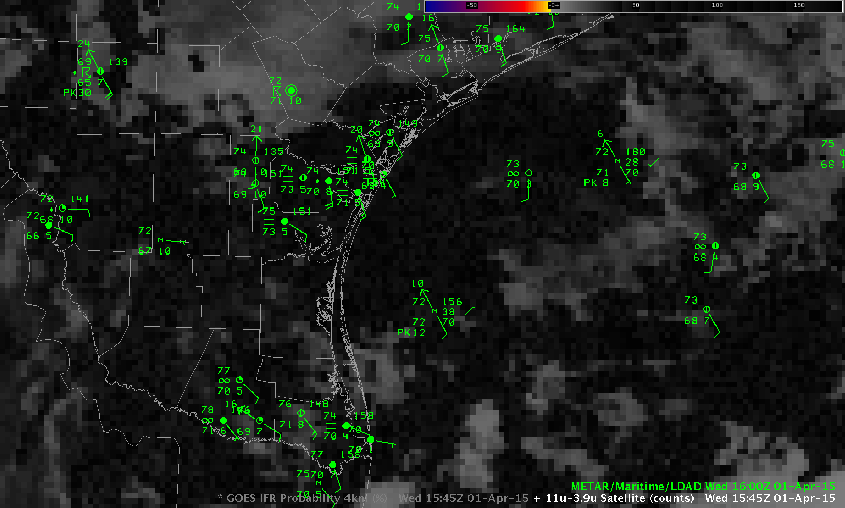
GOES-East Brightness Temperature Difference Field, 1545 UTC on 1 April 2015 (Click to enlarge)
A similar event occurred in March 2015 along the Florida Atlantic Coast. (Link).