Monthly Archives: March 2015

Dissipation Time

CloudThickness_1115_31March2015

GOES-R Cloud Thickness over southern Georgia/northern Florida, 1115 UTC on 31 March 2015 (Click to enlarge)

If fog has formed via radiational cooling, the GOES-R Cloud Thickness product that is produced just before sunrise can be used to estimate when clouds will clear. Such an image is shown above for a case of dense fog over southern Georgia on 31 March 2015. The largest Cloud Thicknesses at this time were around 1150 feet over the southern part of this region. Based on this correlation curve, then, dissipation where the fog is thickest should occur 4-1/2 to 5 hours after 1115 UTC. The visible animation below suggests that dissipation was complete by 1715 UTC.

VIS_1630to1730_31March2015

Visible Imagery, 1630-1815 UTC on 31 March 2015 (Click to enlarge)


Fog over Western Oregon

GOES_IFR_26March2015_05to17z

GOES-R IFR Probabilities computed from GOES-15, hourly from 0500 through 1700 UTC, 26 March 2015 (Click to enlarge)

GOES-R IFR Probabilities during the morning of 26 March 2015 expanded eastward from the Pacific Ocean as fog and IFR conditions developed over the western quarter of Oregon. At sunrise, IFR Probabilities dropped along the coast in Northwest Oregon, and IFR conditions were not reported at either Tillamook or Newport, but IFR Probabilities remained high in the Willamette and Umpqua River Valleys, where IFR conditions persisted.

The Brightness Temperature Difference Product, below, for the same time shows a signal in regions where fog/IFR conditions were not reported. The use of model data (Rapid Refresh) in the GOES-R IFR Probability algorithm helps screen out regions where low-level saturation is not occurring — either because the clouds detected by the brightness temperature difference are mid-level, or because the brightness temperature difference field is driven by soil-based emissivity differences at 3.9µm and 10.7µm and not cloudiness at all. The brightness temperature difference signal vanishes near sunrise as solar 3.9µm radiation starts to be reflected off clouds; the sign flips after sunrise and the low clouds appear dark.

GOES_BTD_26March2015_05to17z

GOES-15 Brightness Temperature Difference (10.7µm – 3.9µm), hourly from 0500 through 1700 UTC, 26 March 2015 (Click to enlarge)

Both IFR Probabilities and Brightness Temperature Difference fields largely miss the isolated IFR conditions over northeast Oregon, around Baker and Meacham.

Cirrus and IFR Conditions over south Texas

GOES13_BTD_25March2015-01_14z

GOES-13 Brightness Temperature Difference (10.7µm – 3.9µm) Fields, 0100-1400 UTC on 25 March 2015, along with surface observations of ceiling and visibility (Click to enlarge)

GOES-13 Brightness Temperature Difference Fields, above, demonstrate how high and middle clouds can complicate or prevent the detection of low clouds from satellite. The beginning of the animation shows signatures of cirrus streaking across the northern part of the domain. There are also signals of low clouds/fog over south Texas that diminish by ~0300 UTC before reappearing. No fog is reported during the early part of the animation. In the latter half of the animation, cirrus moves in to the southern part of the domain from the southwest (cirrus appears black in the enhancement used), interfering with the detection of low clouds and fog over south Texas. At 1400 UTC, the end of the animation, reflected 3.9µm radiation originating from the rising sun has flipped the sign of the brightness temperature difference field.

GOES13_IFRPROB_25March2015_01_14z

GOES-13-based IFR Probability Fields, 0100-1400 UTC on 25 March 2015, along with surface observations of ceiling and visibility (Click to enlarge)

The GOES-R IFR Probability fields, above, show little signal until after 0500 UTC when the satellite and model data both start to suggest the presence of fog/low stratus.  When the cirrus impinges on the southern part of the domain, becoming noticeable at 1000 UTC, IFR Probability values drop because satellite predictors cannot be used in the algorithm — only model data is driving the field over south Texas.  The model data strongly suggests fog is present however (and IFR and near-IFR conditions are reported).  Using the fused product allows a forecaster to have a consistent signal as the high clouds move in.  IFR conditions persist — and IFR Probabilities remain high — after sunrise over portions of south Texas.

Fog under high clouds

IFRBTD_1100UTC_16March2015

Early morning March 16 2016 had another fine example of the importance of using fused information to detect regions of low clouds and fog. The animation above shows the Brightness Temperature Difference (10.7µm – 3.9µm) and IFR Probability fields from 1100 UTC 16 March 2016. A cirrus canopy over Texas and Louisiana prevents the satellite from detecting radiation emitted from lower clouds. In this region, the IFR Probability field can suggest the presence of fog/low stratus and IFR Conditions because of low-level saturation that is present in the Rapid Refresh Model. Fusing this information together allows for a better depiction of where IFR Conditions are present. Cirrus clouds are not present over Arkansas; there, both satellite and model can be used to compute IFR Probabilities. When both satellite and model suggest fog is present, IFR Probabilities are higher (over Arkansas) than when only model (over Louisiana), or only satellite, suggest fog is present.

When IFR Probabilities suddenly vanish

GOESIFR_PROB_Sunrise_11March2015

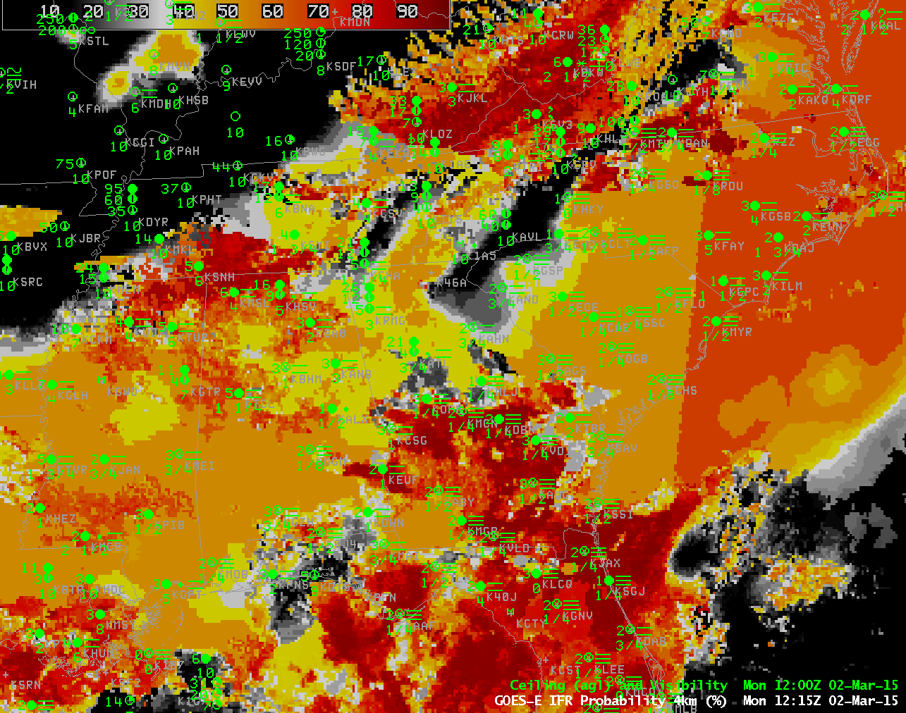
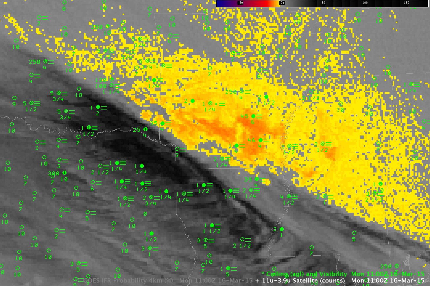
GOES-R IFR Probabilities over Indiana around sunrise on March 11 demonstrated what can happen when the Cloud Mask does not detect clouds, for whatever reason. The three-image loop above shows GOES-R IFR Probability at 1230, 1315 and 1330 UTC on 11 March. In the 1230 UTC image, the boundary between daytime predictors (to the east) and nighttime predictors (to the west) is manifest as a nearly north-south line through Kentucky and eastern Indiana. At 1315 UTC, a different boundary has appeared central lower Michigan, and this boundary moves westward to central Illinois at 1330 UTC. IFR Probabilities drop quickly to ~2% as this boundary passes, even though widespread IFR conditions are apparent. What is going on?

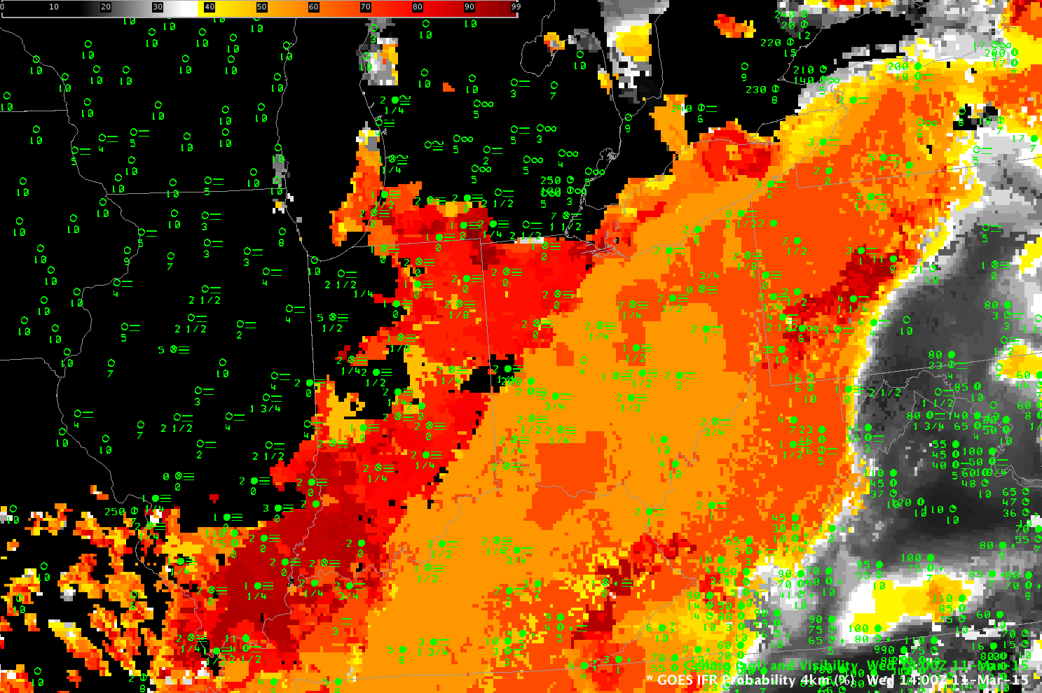
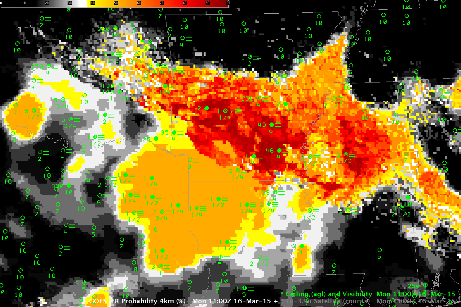
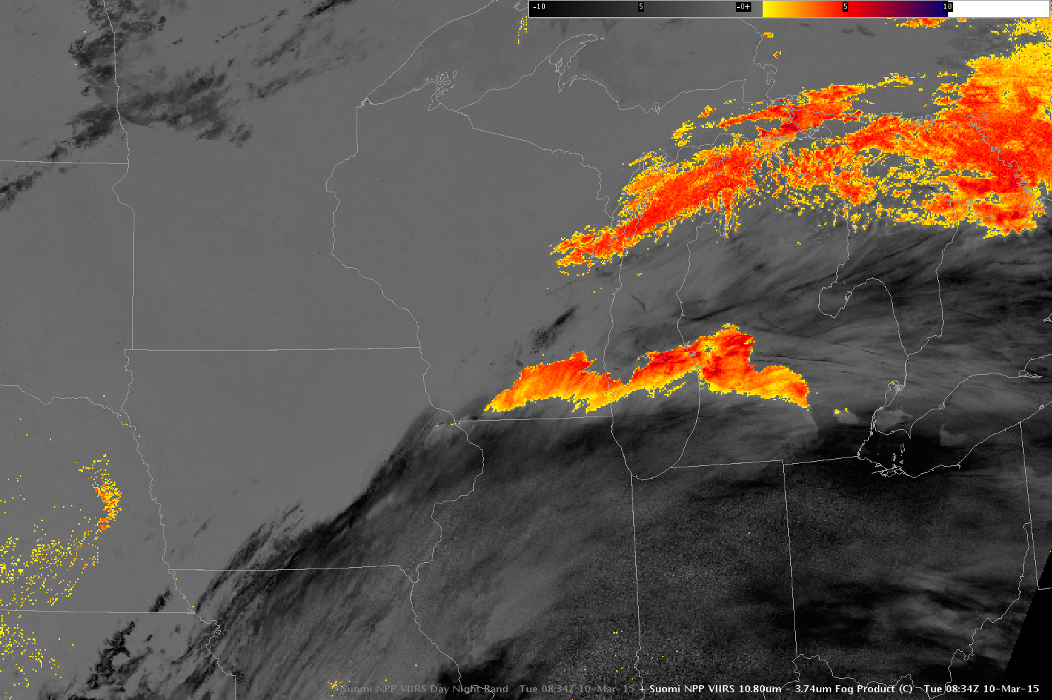
In this case, the cloud mask algorithm has failed to identify clouds over Indiana where clouds are present. A lack of clouds suggests Fog cannot be present. During the night, cloud masking is assigned less weight (because cloud detection is more difficult at night) so the cloud mask has a smaller impact on the IFR Probability. As night transitions into day, however, cloud masking acquires more importance in the computation of IFR Probability so the lack of a cloud will greatly influence IFR Probabilities. The IFR Probability algorithm also has a temporal check, so the effect of no cloud — as determined by the cloud mask — does not happen immediately as the sun rises. The animation below of cloud type shows no cloud type detected (starting at 1215 UTC over Michigan) in the regions where IFR Probabilities dropped. (That is, the cloud mask says no cloud is present; note also how IFR Probabilities do persist with the supercooled clouds over lower Lake Michigan, and with the clouds over southern Illinois).  Notice also how the cloud type returns over southern Illinois at 1315 UTC — the cloud mask is more accurate at that point.  Cloud masking identifies clouds over most of Indiana and Illinois by 1400 UTC; this can be deduced by the presence of cloud type values there.  The 1400 UTC GOES-R IFR Probability field, at bottom, shows IFR Probabilities redeveloping over Indiana and Illinois.

The Cloud Mask that is used by GOES-R IFR Probabilities is scheduled to be replaced with a more accurate (and more up-to-date) Bayesian Cloud Mask in the near future. This change, and GOES-R data (GOES-R is scheduled to launch on March 11 2016, in one year) will likely mitigate such cloud-masking errors as occurred on March 11 2015.

geocat.GOES-EAST.2015070.104500.to.143000.WISC.ctypeloop

GOES-13 Cloud Type, 1045 – 1430 UTC on 11 March 2015 (Click to enlarge)

GOES_IFRPROB_1400UTC_11March2015

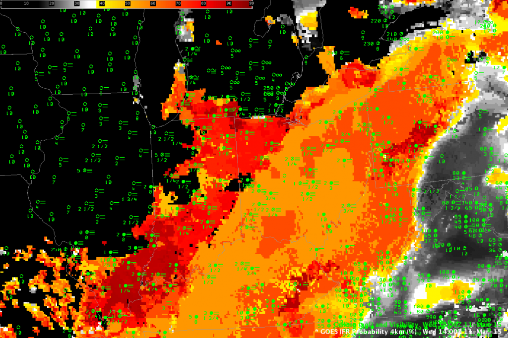
GOES-R IFR Probabilities, 1400 UTC 11 March 2015 (Click to enlarge)

Fog under high clouds over the Midwest

IFRPROB_UpperMidwest_10March2015_2_11

GOES-R IFR Probability Fields, 0200-1100 UTC on 10 March 2015, along with surface observations of ceilings and visibilities (Click to enlarge)

A region of dense fog/low clouds moved northward overnight through Illinois and into Wisconsin. Its movement northward was captured accurately by the GOES-R IFR Probability fields, above. IFR conditions develop as the region of high IFR Probability moves overhead. In addition, as the IFR Probability fields move northward, ceilings and visibilities along its southern flank improve. That is, the IFR Probability fields capture the northward motion of improving visibilities over Illinois. Detecting when visibilities improve is as important as detecting when visibilities deteriorate, and the GOES-R IFR Probability field in this case is doing both.

Compare that to the traditional method of detecting low clouds, the brightness temperature difference field, shown below. Low stratus and fog along the northern edge of the cirrus shield is detected, but the northward movement of the southern edge of the IFR conditions cannot be detected under the cirrus.

BTD_1100_10March2015_7_11

GOES-East Brightness Temperature Difference Fields (10.7µm – 3.9µm), 0700-1100 UTC, 10 March 2015 (Click to enlarge)

Suomi-NPP overflew the region at 0830 UTC, just as the fog was moving into southern Wisconsin. The image below shows the extensive cloud field.  The brightness temperature difference field (11.32µm – 3.74µm) (here) for the same time suggests that much of the cloudiness detected over Illinois is higher cloud.

SNPP_DNB_0834_10March2015

Suomi NPP Day Night Band (0.70 µm) imagery, 0334 UTC on 10 March 2015 (Click to enlarge)

IFR Probabilities with a developing storm system

GOES_IR4_09March2015_0630UTC

GOES-East 10.7 µm imagery at 0630 UTC on 9 March 2015 (Click to enlarge)

The 10.7 µm imagery from GOES-East (Band 4) shows a cloud signature that is typical of a developing low-pressure system that one might find to the east of an open wave at 300 mb. Using satellite data alone to deduce (or perceive) the presence of IFR conditions in this case will be difficult. GOES Sounder Estimates of Total Precipitable Water in the region (from here) give little information.

GOES-R IFR Probability fields blend together satellite information with moisture information from the Rapid Refresh (also included: slowly varying fields such as Sea Surface Temperature and surface emissivity). The animation below, showing the field at 0615, 0915 and 1215 UTC, demonstrates the product’s ability to distinguish between regions with cloud (Louisiana) and regions with fog/low stratus (Much of east Texas, stretching up into central Arkansas; observations show IFR or near-IFR conditions widespread in this area). Because satellite data are unavailable for the product (only water-based cloud information is used, typically, and multiple cloud layers associated with deep clouds include mixed phase and ice clouds) the fields are fairly uniform. Where holes in the clouds appear — over the Rio Grande at 0915 UTC and over parts of south Texas at 1215 UTC — IFR Probabilities look more pixelated and Probabilities are higher. The larger IFR Probabilities occur because satellite predictors are incorporated into the algorithm where low clouds are detected.

IFR_PROB_09March2015_6_9_12

GOES-R IFR Probability fields and surface plots of ceiling/visibility and the NWS Frontal Analysis at ~0600, ~0900 and ~1200 UTC on 9 March (Click to embiggen)

Fog over the High Plains of Texas

GOES_IFR_PROB_20150303_0400_1000

GOES-R IFR Probability Fields, hourly from 0400 through 1000 UTC on 3 March 2015 (Click to enlarge)

Persistent fog has shrouded the High Plains of Texas for the past couple days.  GOES-R IFR Probability fields, above, from 0400 to 1000 UTC on 3 March, show the widespread nature of the fog.  There are regions in the animation (north and west of San Angelo at the start of the loop and north and west of Midland at the end of the loop) where the character of the IFR Probability field (a uniform value with a flat field and orange color) suggests high clouds are present and that fog detection with the product is relying on Rapid Refresh model output.  That the GOES-R IFR Probability fields align well with observations of IFR or near-IFR conditions is testimony to the accuracy of the Rapid Refresh Model. In the southern part of the domain, where GOES-R IFR Probability values are larger (the field is red), satellite data are also used in the computation of the IFR Probability field. Because satellite predictors can also be used there, confidence that fog/low stratus exists is greater, and the IFR Probability field values are larger. Note that the IFR Probability field there is also pixelated, reflecting the small pixel size (nominally 4 km) of the GOES Imager.

VIIRS_DNB_FOG_20150303_0905

Suomi NPP Brightness Temperature Difference Field (11.35 µm – 3.74 µm) and Day Night Band (0.70 µm) at 0905 UTC on 3 March 2015 (Click to enlarge)

Suomi NPP and Aqua both overflew the region around 0900 UTC on 3 March, and the high-resolution snapshots from Suomi NPP (above) and MODIS (below) show scenes that agree with the GOES Imagery. The Brightness Temperature Difference Fields show middle and high clouds over the Texas Panhandle. The Day Night band shows clouds over most of Texas — but it is difficult to distinguish high clouds and low clouds from the imagery. Shadows can be used to infer differences in cloud height — but that requires a knowledge of where the Moon sits in the sky relative to Texas at this time: to the east, or to the west?

The MODIS-based GOES-R IFR Probability field at ~0900 UTC, below, again shows how model data is helpful in filling in regions where high clouds or mid-level clouds obscure the satellite-view of low clouds/stratus.

MODIS_FOG_IFR_PROB_20150303_0855

MODIS-based GOES-R IFR Probability and Aqua Brightness Temperature Difference Fields (11 µm – 3.9 µm) at 0855 UTC, 03 March 2015 (Click to enlarge)

IFR Conditions over the Southeast United States

US_11-3.9_Sat_20150302anim

Brightness Temperature Difference Fields (10.7µm – 3.9µm) from GOES-East, hourly from 0400-1300 UTC on 2 March 2015 (Click to enlarge)

A series of frontal systems along the east coast caused multiple cloud layers and IFR conditions over much of the deep south and piedmont from Mississippi to Georgia and up through Virginia overnight on 1-2 March 2015. The animation of Brightness Temperature Difference (10.7µm – 3.9µm), above, is testimony to the difficulty in using that product as a fog detection device when multiple cloud layers are present: Many stations underneath cirrus show IFR Conditions. (Note also how the signal changes at 1300 UTC — the end of the animation — as the sun rises and increasing amounts of 3.9µm solar radiation is reflected off the clouds).

The GOES-R IFR Probability fields, below, better identify regions of reduced visibility underneath mixed cloud layers. It does this by incorporating model data (from the Rapid Refresh) into its suite of predictors. Thus, where low-level saturation is indicated under multiple cloud layers, IFR Conditions can be assumed to be occurring, and computed IFR Probabilities are large. The hourly animation of GOES-R IFR Probability, below, shows a good overlap between large IFR Probabilities and IFR (or near-IFR conditions). The flat IFR Probability field that is widespread over the Piedmont region of the Carolinas is typical of an IFR Probability field determined mostly by model output. Where high clouds break, pixelated regions develop (and IFR Probabilities increase) in the field.

GOES_IFR_PROB_20150302anim

GOES-R IFR Probability fields, 0400-1300 UTC on 2 March (Click to enlarge)

The 1215 UTC and 1300 UTC imagery in the IFR Probability animation above include a discernible nearly north-south line. (The 1215 UTC image is below).  This is the terminator.  To the right of that line, where IFR Probabilities are slightly larger (dark orange), daytime predictors are being used;  to the left of that line, IFR Probabilities are slightly smaller (lighter orange) and nighttime predictors are being used.  Why is the probability a bit larger in the daytime predictors?  In part this is because visible imagery can be used to ascertain whether clouds are present.  You can be a bit more confident that IFR conditions are present because clouds are present in the visible imagery.

GOES_IFR_PROB_20150302_1215

GOES-R IFR Probability fields, 1215 UTC on 2 March (Click to enlarge)