Category Archives: Stray Light

Fog over ArkLaTex

IFRP-02

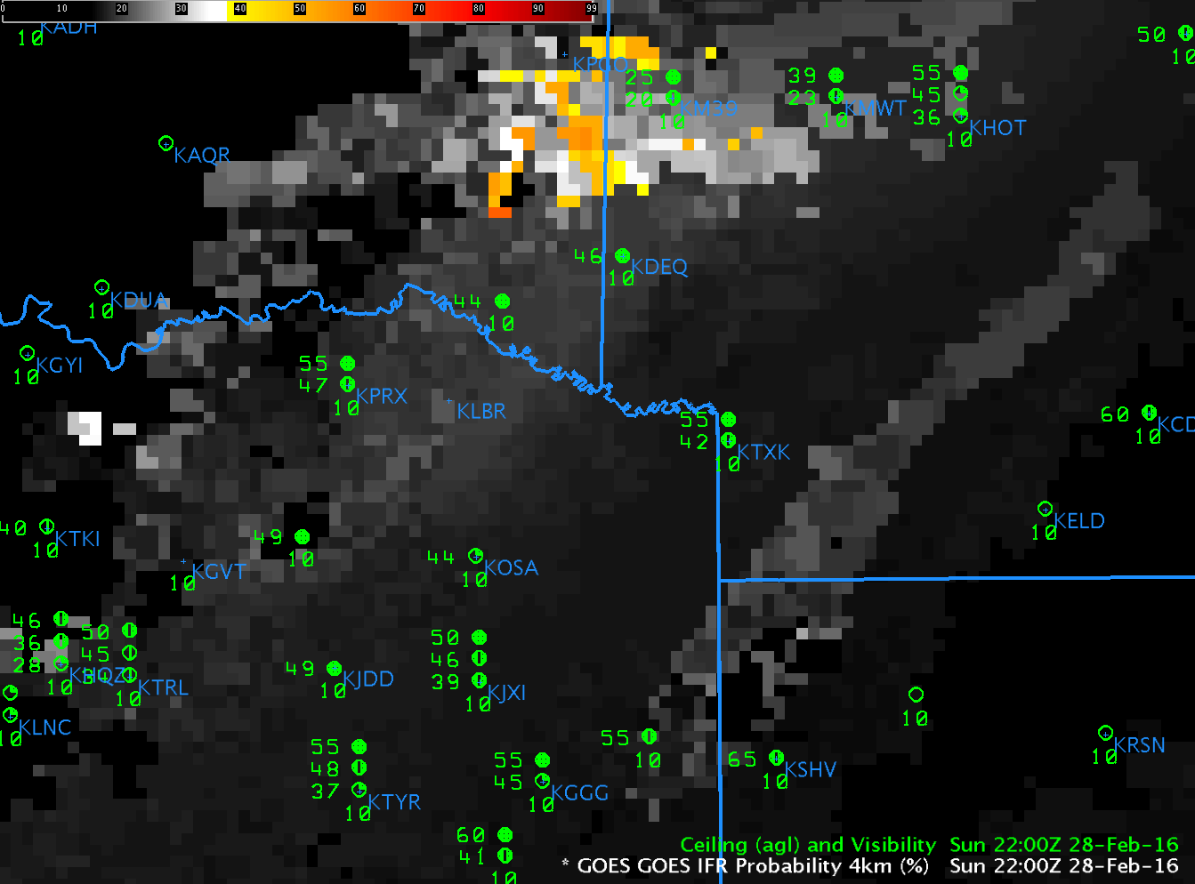
GOES-R IFR Probabilities, 2200 UTC on 28 February 2016 as well as surface observations of ceilings and visibilities (click to enlarge)

Late in the day on 28 February, as shown above, GOES-R IFR Probability fields included a small region of enhancement over west-central Arkansas and east-central Oklahoma. In this case, that field heralded the development of more widespread IFR conditions over northeast Texas (and surroundings). By 0300 on 29 February, below, IFR probailities in the region over east-central Oklahoma/west-central Arkansas had increased, and there is a suggestion of increasing IFR Probabilities over northeast Texas as well.  This is a case where IFR Probabilities can alert a forecaster to pay attention to a region long before a hazard develops.

IFRP-19

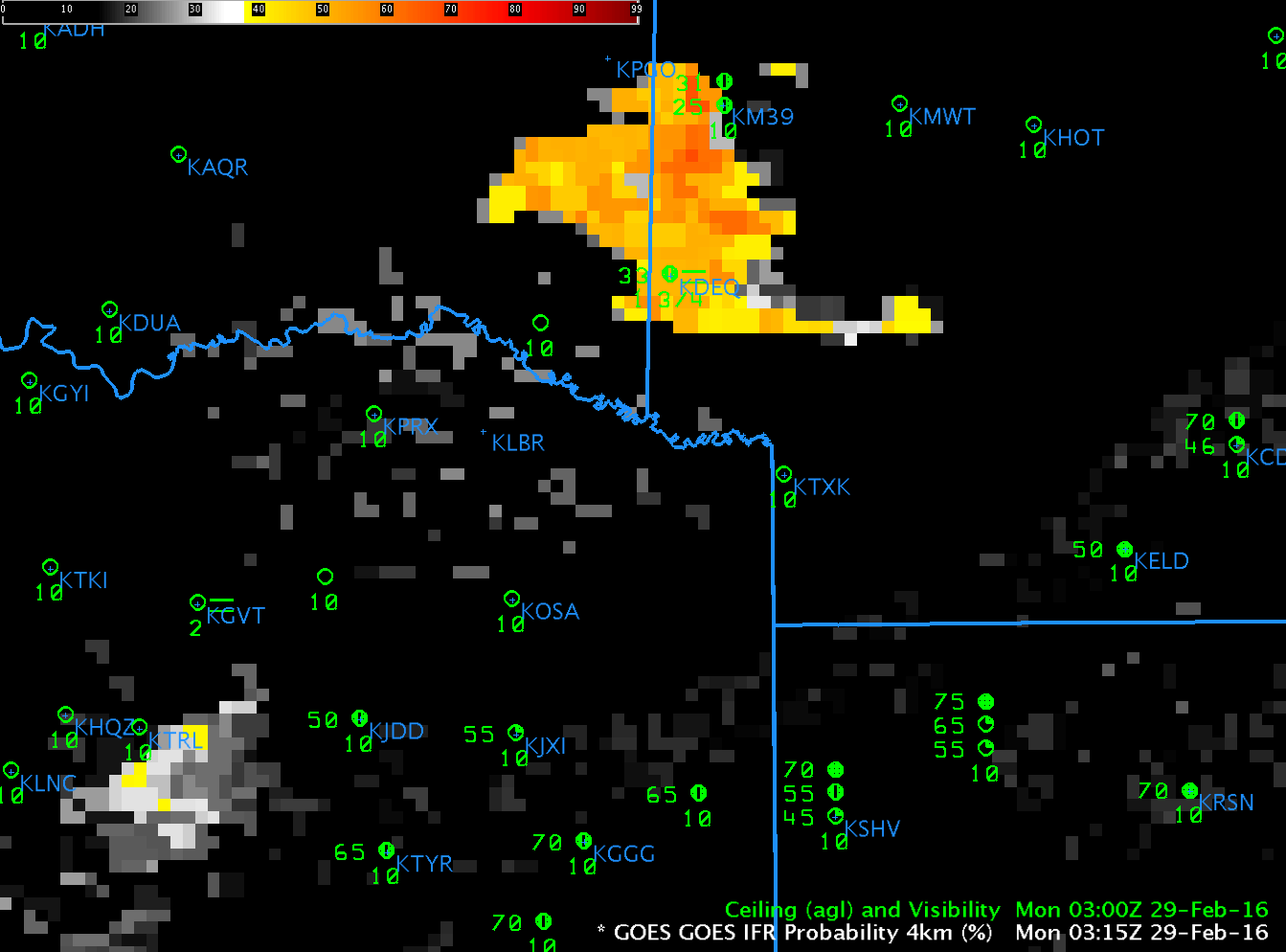
GOES-R IFR Probabilities, 0315 UTC on 29 February 2016 as well as surface observations of ceilings and visibilities (click to enlarge)

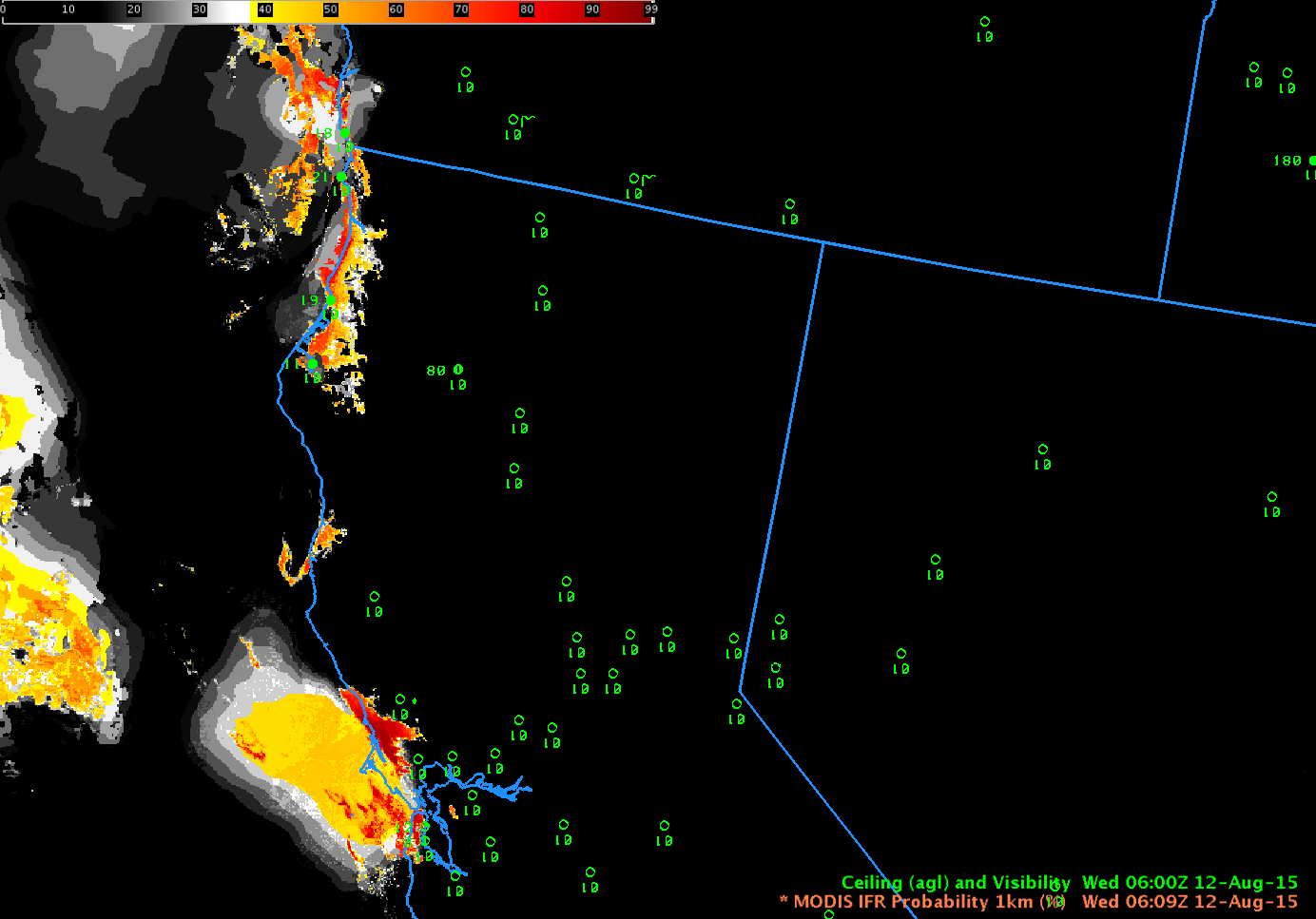
Late February starts the time when GOES-13 is near enough to eclipse season that stray light can creep into imagery. In this case, a large signal increase between 0500 and 0515, below, is in part related to stray light, and in part to low cloud development. By 0530, IFR Probability fields show less affect from stray light. (Click here for an animation of brightness temperature difference fields alone; Stray Light has an obvious impact at 0515 UTC).

IFR_P_0500_0530_29feb2106anim

GOES-R IFR Probability fields, 0500-0530 UTC, 29 February 2016, showing Stray Light Effects (Click to enlarge)

IFR Probability fields from 0615 through 1215 UTC are shown below. Very high IFR Probabilities (and IFR conditions) were widespread in the early morning over northeast Texas and surrounding states.

IFRPanim_0615_1215_29February

GOES-R IFR Probabilities fields, hourly from 0615-1215 UTC, and surface reports of ceilings and observations (Click to enlarge)

Dense Fog over central Nebraska

Nebraska_18August2015_0315_1100anim

GOES-R IFR Probability (Upper Left), GOES-R Low IFR Probability (Lower Left), GOES-13 Brightness Temperature Difference Field (10.7 µm – 3.9 µm) (Upper Right), GOES-R Cloud Thickness (Lower Right), Times as Indicated (Click to enlarge)

GOES-R IFR Probability fields, above, suggest IFR conditions are developing over central Nebraska during the early morning of 18 August 2015. Several aspects of the field require comment. At the beginning of the animation, there are noticeable north-south oriented lines in the IFR and Low-IFR Probability fields. These are artifacts of determining the saturation in the lowest 1000 feet of the model as discussed here. As the model saturation deepened over the course of the night, those parallel lines disappeared.

The flat nature of the field announces that satellite data are not being used in the computation of IFR Probability because multiple cloud layers are present. Model fields lack the fine spatial resolution of GOES Satellite data. Where breaks in the clouds do occur, GOES-R IFR Probability fields increase in value (because cloud predictors can be used, and their use enhances the ability of the algorithm to predict whether fog/low clouds are present): Temper your interpretation of the magnitude of the IFR Probability with knowledge of presence of clouds.

Note that the Brightness Temperature Difference field at 0500 UTC has much larger values. Stray Light is beginning to impinge on satellite fields as the calendar gets closer to the Equinox. This issue will remain through mid-October. Multiple cloud decks over Nebraska on 18 August greatly hampered the ability of the brightness temperature difference field to identify regions of low clouds.

The GOES-R Cloud Thickness fields are displayed; these are derived from an empirical relationship between 3.9 µm emmissivity and cloud thickness derived from SODAR data off the west coast of the United States. When multiple cloud layers are present, this field is not computed (nor is it displayed around sunrise/sunset). Thus, you should not see Cloud Thickness fields in regions where GOES-R IFR Probability fields are very smooth (suggesting that only model data are being used). The regions where Cloud Thickness is displayed, above, correspond to regions in the IFR Probability field that are pixelated (that is, where satellite data are being used).

Fog formation is aided by increasingly long nights. Nights now are above 90 minutes longer in Hastings than they were at the Summer Solstice.

HastingsNE

The text for the advisory is below:

URGENT - WEATHER MESSAGE
NATIONAL WEATHER SERVICE HASTINGS NE
608 AM CDT TUE AUG 18 2015

...DENSE FOG PERSISTING FOR A FEW HOURS THIS MORNING...

NEZ048-049-061>064-073>077-181400-
/O.NEW.KGID.FG.Y.0006.150818T1108Z-150818T1400Z/
MERRICK-POLK-BUFFALO-HALL-HAMILTON-YORK-PHELPS-KEARNEY-ADAMS-CLAY-
FILLMORE-
INCLUDING THE CITIES OF...CENTRAL CITY...STROMSBURG...OSCEOLA...
SHELBY...POLK...KEARNEY...GRAND ISLAND...AURORA...YORK...
HOLDREGE...MINDEN...HASTINGS...SUTTON...HARVARD...CLAY CENTER...
EDGAR...FAIRFIELD...GENEVA...EXETER...FAIRMONT
608 AM CDT TUE AUG 18 2015

...DENSE FOG ADVISORY IN EFFECT UNTIL 9 AM CDT THIS MORNING...

THE NATIONAL WEATHER SERVICE IN HASTINGS HAS ISSUED A DENSE FOG
ADVISORY...WHICH IS IN EFFECT UNTIL 9 AM CDT THIS MORNING.

* VISIBILITY...REDUCED TO 1/4 MILE OR LESS ACROSS MUCH OF THE
  ADVISORY AREA...INCLUDING THE INTERSTATE 80 AND HIGHWAY 6
  CORRIDORS. THE COMBINATION OF RAIN MOVING INTO PARTS OF THE
  AREA...ALONG WITH A COLD FRONT MOVING IN FROM THE WEST...SHOULD
  HELP TO GRADUALLY IMPROVE DENSE FOG ISSUES.

* IMPACTS...DENSE FOG WILL GREATLY AFFECT THE MORNING COMMUTE IN
  SOME AREAS...AND MOTORISTS ARE URGED TO DRIVE WITH CAUTION AND
  PREPARE FOR RAPID CHANGES IN VISIBILITY OVER SHORT DISTANCES.

PRECAUTIONARY/PREPAREDNESS ACTIONS...

A DENSE FOG ADVISORY MEANS VISIBILITIES WILL FREQUENTLY BE
REDUCED TO LESS THAN ONE QUARTER MILE. IF DRIVING...SLOW DOWN...
USE YOUR HEADLIGHTS...AND LEAVE PLENTY OF DISTANCE AHEAD OF YOU.

&&

$$

PFANNKUCH

Coastal California Fog

NPP_DNB_BTD_1003UTC_12August2015toggle

Toggle between Suomi NPP Day Night Band Visible (0.70 µm) Image and Brightness Temperature Difference (11.45 µm – 3.74 µm) , 1003 UTC 12 August 2015 (Click to enlarge)

Suomi NPP data from 1003 UTC on 12 August, above, shows evidence of a cloud bank hugging the northern California coast from Cape Mendocino to San Francisco Bay. It also penetrates inland to Santa Rosa in Sonoma County. (Note also how the fires burning in interior show up well in the Day Night Band — they are emitting visible light — and in the Brightness Temperature Difference band — because they are much warmer in the 3.74 µm image than in the 11.45 µm image).

Terra overflew the California coast at ~0600 UTC and Aqua overflew the coast at ~1000 UTC; MODIS-based IFR Probabilities could be constructed from these overpasses, and they are shown below.  At 0609 UTC, High IFR Probabilities (>90%) are confined to coastal Sonoma County and along the coast from Humboldt county north.  By 1023 UTC, high IFR Probabilities stretch along the entire coast from Cape Mendocino to the mouth of San Francisco Bay, with evidence of inland penetration along river valleys.  (The Russian River, for example, and perhaps the Noyo River in Mendocino County)

MODIS_IFR_0609UTC_12August2015

Terra MODIS-based GOES-R IFR Probability fields, 0609 UTC, 12 August 2015 (Click to enlarge)

MODIS_IFR_1023UTC_12August2015

Aqua MODIS-based GOES-R IFR Probability fields, 1023 UTC, 12 August 2015 (Click to enlarge)

MODIS can give high-resolution imagery, but the infrequency of the scenes tempers its usefulness. In contrast, GOES-15 (as GOES-West) views the California coast every 15 minutes, and this excellent temporal resolution (that will improve in the GOES-R era) allows a better monitoring of the evolution of coastal fog. Hourly plots of GOES-R IFR Probability, below, computed from GOES-15 and Rapid Refresh Data show the slow increase in GOES-R IFR Probabilities along the coast as ceilings and visibilities drop.

GOESWIFR_12August2015_0400_1200anim

GOES-R IFR Probability fields, 0400-1200 UTC 12 August 2015 (Click to enlarge)

In the animation above, note the general increase in GOES-R IFR probabilities at 0900 UTC relative to 0800 and 1000 UTC. We are close enough to the Solstice that Stray Light Issues are starting. The 0800, 0900 and 1000 UTC brightness temperature difference imagery, below, shows the large signal increase at 0900 UTC that can be attributed to stray light. GOES-R IFR Probabilities can tone down that increase somewhat — because the model data will now show low-level saturation in regions where stray light erroneously suggests low clouds/fog might exist. GOES-R IFR Probabilities also screen out the constant fog signal over the Central Valley of California (and over Nevada) that is driven not by the presence of low clouds but by soil emissivity differences.

GOESWBTD_12August2015_0800_0900_1000step

GOES-15 Brightness Temperature Difference (10.7 µm – 3.9 µm), 0800, 0900 and 1000 UTC 12 August 2015 (Click to enlarge)


======================== Added =========================
GOES-14 in SRSO-R mode (see also this link) viewed the west coast starting at 1115 UTC today. The Brightness Temperature Difference field, below, (click here for mp4) shows the slow expansion/evaporation of the low stratus/fog. (GOES-R IFR Probabilities were not computed with the GOES-14 1-minute imagery). The rapid change in the field at sunrise occurs because solar radiation at 3.9 µm quickly changes the brightness temperature difference from negative to positive.

Visible Imagery is below (Click here for mp4).

960x1280_AGOES14_B1_GOES14_W_animated_2015224_133000_182_2015224_170000_182_GRAY

GOES-14 Visible Imagery (1330-1700 UTC) (Click to animate)

Fog over the Ozarks and southern Plains

GOES_IFR_21Oct2014_01-13

GOES-IFR Probabilities, computed from GOES-13 and Rapid Refresh, hourly from 0100 through 1300 UTC on 21 October 2014 (Click to enlarge)

Fog and stratus developed overnight over the Ozark Mountains and southern Plains. The hourly loop of GOES-R IFR Probabilities shows the development and expansion of visibility and ceiling reductions over the area. How do these fields compare to other measures of fog? Brightness Temperature Difference fields, below, generally overestimate the regions of fog. The 0200 and 0800 UTC brightness temperature difference fields, below, are toggled with the IFR Probabilities; the inclusion of surface information via the Rapid Refresh Model correctly limits the positive brightness temperature difference to regions where fog and low stratus are most likely. The satellite-only signal overpredicts regions of reduced visibilities because it can only see the top of the cloudbank; this offers little information about the cloud ceilings!

GOES_BTD_IFR_0200_21Oct2014_toggle

GOES-13 Brightness Temperature Difference (10.7 µm – 3.9 µm) and GOES-based IFR Probabilities at 0200 UTC, 21 October 2014 (Click to enlarge)

GOES_BTD_IFR_0800_21Oct2014_toggle

GOES-13 Brightness Temperature Difference (10.7 µm – 3.9 µm) and GOES-based IFR Probabilities at 0800 UTC, 21 October 2014 (Click to enlarge)

Brightness Temperature Difference fields are occasionally contaminated by stray light in the signal. This happened on 21 October at 0400 UTC. The Brightness Temperature Difference fields at 0345, 0400 and 0415 UTC are shown below, with the GOES-R IFR Probabilities for the same time follow. Note how Stray Light contamination does bleed into the GOES-R IFR Probability field; if there is a large change over 15 minutes in the IFR Probability signal, consider the possible reasons for that change. Stray light contamination is a strong candidate if the signal is near 0400-0500 UTC with GOES-East. There are regions in the IFR Probability fields where even the strong — but meteorologically unimportant — brightness temperature difference signal during stray light is not enough to overcome the information from the Rapid Refresh model that denies the possibility of low-level saturation (for example, in northern Kansas or southern Oklahoma).

GOES_BTD_21Oct2014_0345-0415

GOES-13 Brightness Temperature Difference (10.7 µm – 3.9 µm) at 0345, 0400 and 0415 UTC, 21 October 2014 (Click to enlarge)

GOES_IFR_21Oct2014_0345-0415

GOES-based IFR Probabilities at 0345, 0400 and 0415 UTC, 21 October 2014 (Click to enlarge)

MODIS data from either Terra or Aqua can give important early alerts to the development of Fog/Low Stratus. Because of its superior resolution to GOES, the character of the developing fog can be depicted with more accuracy. The MODIS-based IFR Probability, below, in a toggle with the GOES-based IFR Probability at the same time, distinctly shows that the fog development at 0430 UTC is starting in the small valleys of the Ozarks of northwest Arkansas. GOES-based IFR Probabilities give a broader signal; certainly if you are familiar with the topography of the WFO you can correctly interpret the coarse-resolution GOES data, but the MODIS data spares you that necessity.

MODIS_GOES_IFR_21Oct2014_0430

GOES- and MODIS-based IFR Probabilities at ~0430 UTC, 21 October 2014 (Click to enlarge)

Suomi NPP data can also be used to compute IFR Probabilities, but those data are not yet computed for AWIPS. The Ozarks were properly positioned on 21 October to be scanned by two successive orbits of Suomi NPP (one of the benefits of Suomi NPP’s relatively broad scan), and the brightness temperature difference fields (11.45µm – 3.74µm) at 0715 and 0900 UTC are shown below. As with MODIS, the strong signal in the river valleys is apparent. (The Day Night band from Suomi NPP for this event does not show a strong signal because the near-new Moon provides no illumination at 0745 or 0900 UTC: it hasn’t even risen yet.)

SNPP_BTD_21Oct2014_0715-0900

Suomi NPP Brightness Temperature Difference (11.45 µm – 3.74 µm) and 0715 and 0900 UTC, 21 October 2014 (Click to enlarge)

Stratus/Low Clouds with developing Storms on the Plains

GOES_IFR_PROB_20131029loop

GOES-13-based GOES-R IFR Probabilities (Upper Left), GOES-13 Brightness Temperature Difference Product (10.7 µm – 3.9 µm) (Upper Right), GOES-R Cloud Thickness (Lower Left), Suomi-NPP Day/Night band (Lower Right), all times as indicated (click image to animate)

The ongoing change of seasons means that stronger large-scale weather systems are more likely. When something like a Colorado Cyclone moves from the Rockies and emerges into the central part of USA, it brings multiple cloud layers with it, and those many cloud layers make detection of fog and low stratus difficult. The animation above shows GOES-R IFR Probabilities and Cloud Thicknesses as well as the color-enhanced GOES-13 Brightness Temperature Difference (BTD) field. Note the characteristic signal in the BTD field of jet-level cirrus over Kansas. In these regions, BTD fields cannot be used to diagnose regions of low-level clouds because the upper-level clouds block the satellite view of lower clouds.

IFR Probability does have a signal over Kansas, however (where IFR conditions are present — see the animation below). Rapid Refresh data are being used under the cirrus to diagnose the probability of IFR conditions. Thus, IFR Probability fields are filled in under regions of high cirrus. Because only model data are being used to diagnose IFR Probability fields over central and southern Kansas, the characteristic of the field is different. Where satellite and model data are used, as over western Nebraska, the IFR Probability field has a pixelated appearance; where only model data are used, as over southern Kansas, the IFR probability field has a very smooth appearance. In model-only regions, in addition, IFR Probabilities are smaller because the number of predictors available to the algorithm is smaller.

The BTD field highlights regions in eastern Nebraska as having water-based clouds? Are these clouds causing low ceilings and reduced visibilities? No, and IFR probabilities in that region are low. In this region, Rapid Refresh data do not show low-level saturation, and thus the IFR Probabilities are correctly small, despite the strong satellite signal.

GOES_IFR_PROB_20131029withobs_loop

GOES-13-based GOES-R IFR Probabilities and surface visibilities/ceilings, all times as indicated (click image to enlarge)

GOES-R Cloud Thickness, shown at top, is only computed in regions where the highest cloud detected by the satellite is water-based; the algorithm considers includes information from a cloud-typing algorithm, and if clouds are ice phase (or mixed phase) as is likely in the case of jet stream cirrus, cloud thickness is not computed. (Cloud Thickness is also not computed during times of twilight — that is, an hour or so on either side of sunrise and sunset).

GOES_IFR_PROB_20131029_straylightloop

As above, but for a case of Stray Light, all times as indicated (click image to enlarge)

There are still cases at night when Stray Light will contaminate/enhance the 3.9 µm signal on GOES-13, and this contamination can propagate into the GOES-R IFR Probability of Cloud Thickness Fields. In this case, only the Cloud Thickness Fields are affected (below); Cloud thickness jumps about 500 feet for one time period (0415 UTC).

Cold frontal passage in Oregon

GOES-R IFR Probabilities (Upper Left), GOES-West Brightness Temperature Difference (10.7 µm – 3.9 µm) (Upper Right), Topography (Lower Left), GOES-West Water Vapor Imagery (6.7 µm) (Lower Left), hourly from 0400 through 1700 UTC 20 March 2013.

The animation above of the Fog/Low Stratus and Brightness Temperature difference highlights the difficulty that the traditional brightness temperature difference product encounters when multiple cloud layers are present, as you might expect to be present given the water vapor imagery.  At the beginning of the animation, highest IFR probabilities exist over the elevated terrain that surrounds the Willamette Valley in Oregon.  There were also high probabilities off shore.  As the frontal region moves onshore, IFR probabilities increase on shore.   Note also how the GOES-R IFR Probability field is a more coherent one whereas the traditional brightness temperature difference field from GOES contains many separate areas of return that make it harder to see the big picture.  The brightness temperature difference also suffers from stray light contamination at 1000 UTC — but that contamination does not propagate into the GOES-R IFR probability field.

GOES-R IFR Probabilities computed from GOES-West (Upper Left), GOES-West Brightness Temperature Difference (10.7 µm – 3.9 µm) (Upper Right), Topography (Lower Left), Toggle between Suomi/NPP Brightness Temperature Difference (10.8 µm – 3.74 µm) and Day/Night Band, all imagery near 1000 UTC on 20 March 2013

The imagery above shows how straylight contamination in the shortwave IR (3.9 µm) can influence the brightness temperature difference.  The GOES imagery shows the effects (just at this 1000 UTC image, which is also included in the animation above), but that ‘contamination’ does not propagate strongly into the GOES-R IFR Probability.  Note also that the Suomi/NPP Brightness Temperature Difference shows none of the stray light contamination.  Lunar illumination  allows the nighttime visualization of the clouds off the west coast of the US.  As this frontal band moves over Oregon, reduced visibilities result, but only the GOES-R IFR probabilities accurately capture the location of the frontal band because of the multiple cloud layers that exist.

Coastal Stratus over southern California

Hourly imagery of GOES-R IFR Probability computed from GOES-West, from 0200 UTC through 1400 UTC 14 March 2013

Hourly imagery of GOES-R IFR Probability from the overnight/early morning of 14 March 2013 shows the typical advance inland of stratus along coastal southern California.  Several aspects of this loop bear mention.  In the 0200 UTC, the division between daytime predictors (to the left) and nighttime predictors (to the right) is evident extending mostly north-south over the Ocean.  Visibilities at Los Angeles International Airport (LAX) drop to IFR conditions as the diagnosed IFR probabilities push inland.  Note also the good relationship between high probabilities and low visibilities along the coast north of San Diego.

There is a push inland of higher probabilities at 1000 UTC in the loop above that is not well reflected in the observations.  This occurs because of stray light contamination in the brightness temperature difference channel that is obvious in the animation below.  Note also how the many ‘false positives’ in the brightness temperature difference product over land in Southern California, differences that are attributable to emissivity differences in the surface, not to the presence of liquid water clouds, are effectively screened out in the GOES-R IFR Probability product.

Traditional Brightness Temperature Difference product (10.7 µm – 3.9 µm) from GOES-West (mostly).  Note that the ‘seam’ between GOES-East data and GOES-West data is present in the eastern part of the imagery.  Hourly data from 0200 through 1400 UTC on 14 March 2013.

IFR conditions over the upper Midwest

GOES-R IFR Probabilities from GOES-East (Upper Left) at 0832 UTC, along with 0900 UTC observations, Traditional GOES-East Brightness Temperature Difference (10.7  µm – 3.9  µm) at 0832 UTC (Upper Right), GOES-R Cloud Thickness computed from GOES-East (Lower Left), Suomi/NPP Day/Night Band Nighttime visible imagery, 0838 UTC (Lower Left)

Stratus and low clouds persisted over western Minnesota and the eastern Dakotas overnight on 25 to 26 February, and the GOES-R IFR Probability field ably captured the region of lowest visibility.  Note that the IFR probability field extends into northwest Iowa (albeit with relatively lower probabilities).  This is a region where high-level cirrus prevents the traditional brightness temperature difference product from giving useful information about the low levels.  In this region, Rapid Refresh data are used to fill in information and more accurately capture the region of IFR conditions.

As above, but for 0802 UTC for GOES-East Products, and with the MODIS-based IFR probability field at 0801 UTC in the lower left

GOES-R IFR Probabilities can be used with MODIS data as well, and the better resolution (1 km at nadir vs. 4 km at GOES nadir) means the MODIS fields have better small-scale detail.    Note, for exanple, the sharper edge to the IFR probability field in east-central Minnesota.

As at the beginning of the post, except for 0415 UTC (top), 0432 UTC (middle) and 0445 UTC(bottom)

Stray-light issues can influence the 3.9 µm imagery, and therefore the brightness temperature difference field, and therefore the GOES-R IFR Probability field.  In the three images above, Stray Light is noteable in the 3.9 µm at 0432 UTC, but that erroneous information can be de-emphasized in the GOES-R IFR probability field because the Rapid Refresh Data in regions where Stray Light is present may show dryer low levels.

Stray Light in the GOES-R IFR Fog Product

GOES-R IFR Probabilities (upper left), 10.7 µm – 3.9 µm brightness temperature differences (upper right), 3.9 µm micron brightness temperature (lower left), 10.7 µm micron brightness temperature (lower right)

Stray light occasionally intrudes into the 3.9 µm channel, and that has a big impact on both the brightness temperature difference and therefore on the GOES-R IFR product.  The stray light impact on the 3.9 µm channel is evident at 0531UTC — it does not impact the 10.7 µm channel.  The big impact on the brightness temperature difference translates to a big signal in the GOES-R IFR probabilities.  Note how GOES-R IFR probabilities do not change underneath the high-level cirrus over eastern OK, southern MO and Arkansas:  GOES-R IFR probabilities do not use satellite data in regions of multiple cloud layers, or in regions of ice clouds.

Resolution and River Valleys

Animation of GOES-R IFR probabilities (upper left), GOES-R Cloud Thickness (upper right), GOES-East Brightness Temperature Differences (lower left), and Visible Imagery (lower right), from 0400 through 1400 UTC on 6 August 2012

River Valleys — sources of moisture — are nearly sub-pixel scale in GOES-East imagery.  Thus, any signal that develops in a river valley will likely take time to appear, and an example of that occurred over the upper Midwest on the morning of August 6th.  The signal develops along the river starting around 0800 — 0900 UTC (LaCrosse, WI, starts to report visibility and ceiling obstructions at 1000 UTC).  There are several interesting aspects in the loop.

GOES-R IFR probabilities (upper left), GOES-R Cloud Thickness (upper right), GOES-East Brightness Temperature Differences (lower left), and Visible Imagery (lower right), at 0502 UTC on 6 August 2012

The imagery at 0502 UTC (above) shows the result of stray light contamination on the brightness temperature difference field (lower left), but this increase in signal over the Plains is ephemeral, and it is gone in 15 minutes.  There is also an increase in the brightness temperature difference signal over the Plains as sunrise approaches.

GOES-R IFR probabilities (upper left), GOES-R Cloud Thickness (upper right), GOES-East Brightness Temperature Differences (lower left), and Visible Imagery (lower right), at 0915 UTC on 6 August 2012

By 0915 UTC, the GOES-R IFR probabilities have increased slightly along the Wisconsin River in southwest Wisconsin, as has the brightness temperature difference signal (although that signal has increased elsewhere as well where the GOES-R IFR probabilities remain low).  Compare the (relatively) low-resolution GOES-based imagery to the higher resolution Suomi/NPP resolution discussed here.  Note also how the GOES-R IFR probability product correctly suppresses the IFR probabilities over Iowa and Missouri where observations show no obstructions to visibility.