Category Archives: Terrain

Fog in the Mountains

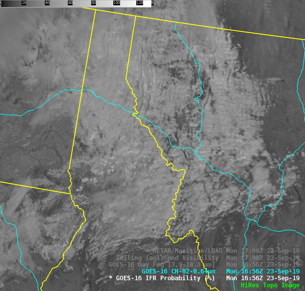
GOES-16 Band 2 (0.64 µm) over Montana and northern Idaho, 1656 UTC on 23 September 2019. Major highways are also shown, including east-west I-90 (Click to enlarge)

Consider the image shown above, visible imagery (0.64 µm) from the GOES-16 Advanced Baseline Imager.    Can you tell at a glance where the IFR Conditions exist?  If you are familiar with northern Rockies topography, and know that the prevailing surface winds in this area were southwesterly, perhaps you can make a good intuitive guess:  low ceilings and reduced visibilities are likely on the upwind side of the topography.

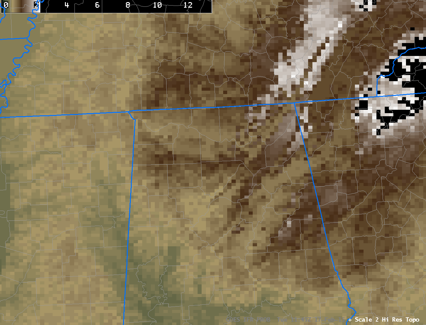
METAR observations at 1700 UTC on 23 September 2019 plotted over topography (Click to enlarge)

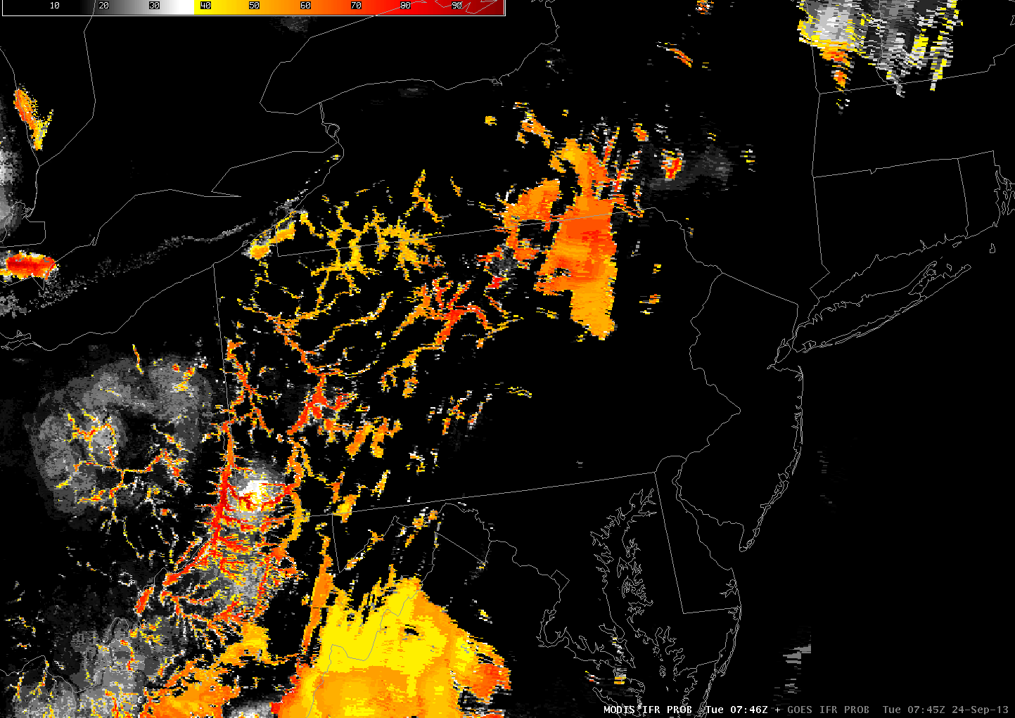
GOES-R IFR Probability fields are computed from visible and infrared imagery as well as from Rapid Refresh model estimates of low-level saturation. IFR Probability fields, below, correctly show increased likelihood of IFR conditions over the mountains, and mostly on the windward side of the topography. Mullan Pass, north of the center of the image, at ~6000 feet above sea level, is observing IFR conditions.

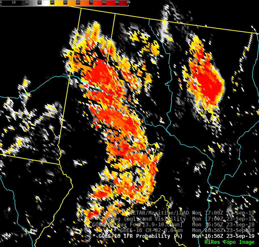
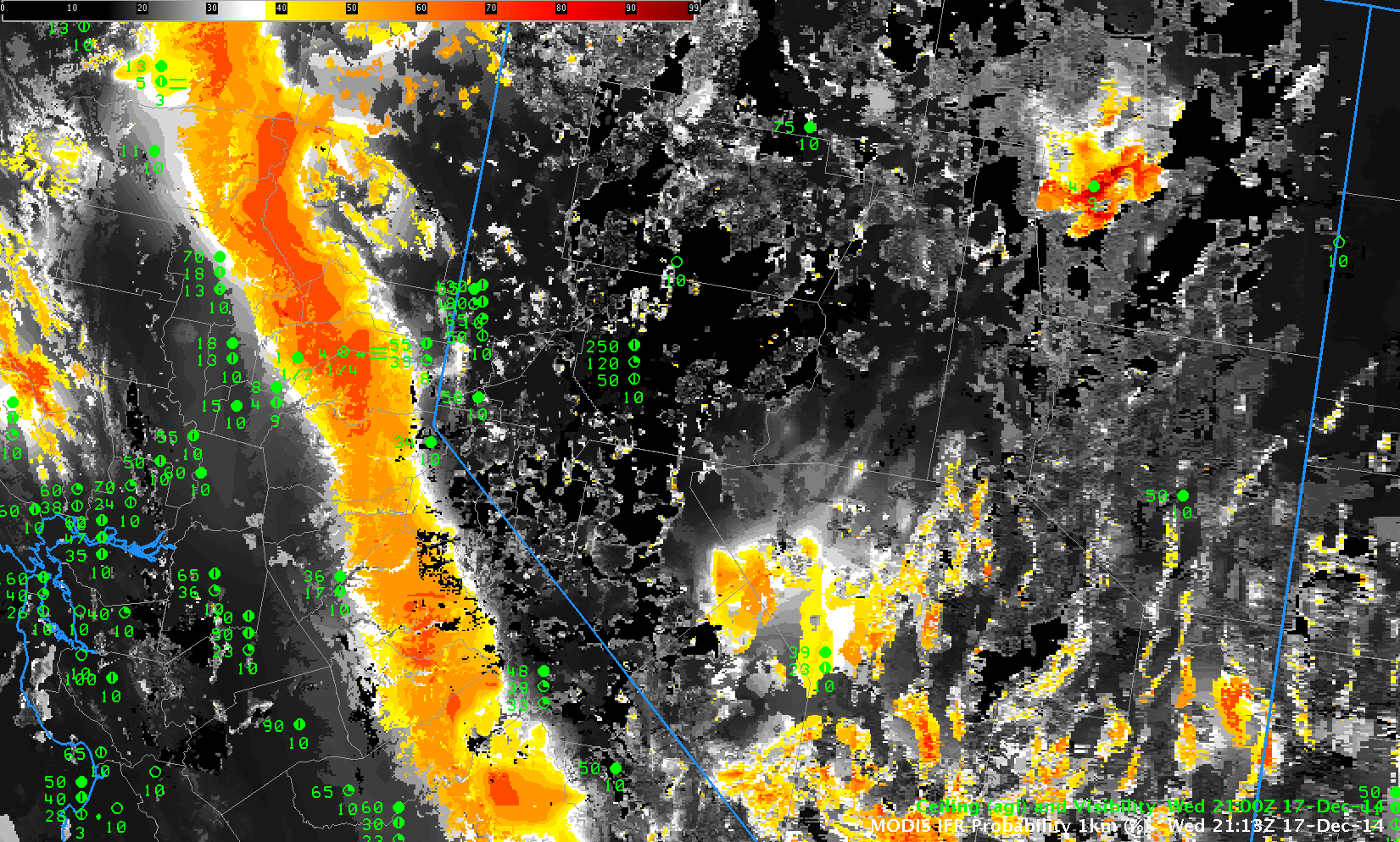
GOES-16 IFR Probability fields, 1656 UTC on 23 September 2019 (Click to enlarge)

The animation below steps through the topography, visible imagery, ‘day fog’ brightness temperature difference (3.9 µm – 10.3 µm) and IFR Probability. The Brightness Temperature Difference field and the visible imagery show little relationship to the IFR Probability field.

Topography, GOES-16 ABI Band 2 (0.64 µm), ‘Day Fog’ Brightness temperature Difference (3.9 µm – 10.3 µm) and IFR Probability fields, all at 1656 UTC on 23 September 2019 (Click to enlarge)

An added benefit of IFR Probability fields: It can be used day or night.

Stratus over Texas

GOES-13 Visible (0.64 µm) Imagery, 1945 UTC on 6 January 2017 and surface observations of ceilings and visibilities (click to enlarge)

Visible imagery over Texas shows an extensive stratus deck blanketing the southern and eastern portions of the state.  Can you tell at a glance — without looking at the observations — if the stratus is extending to the surface?  The animation below shows how GOES-R IFR Probabilities describe the scene, with highest IFR Probabilities offshore (where dense fog is observed over the warm water).  Higher Probabilities also hug the high terrain of eastern Mexico, where IFR conditions are also reported (at Monclova, ID MMMV, where a 500-foot ceiling and 3-mile visibility is reported).  The toggle below cycles through the visible and GOES-R IFR Probability fields and also includes terrain.

GOES-R IFR Probability provides useful situational awareness information during the daytime as well as at night.

GOES-13 Visible (0.64 µm) Imagery, 1945 UTC on 6 January 2017 and surface observations of ceilings and visibilities, and with surface analysis superimposed, as well as GOES-R IFR Probabilities (1945 UTC) and Terrain (click to enlarge)

Multiple Cloud Layers and Topography

IFR_1315_22Apr2016

GOES-R IFR Probability Fields, 1315 UTC on 22 April 2016, along with surface observations of ceilings and visibilities (Click to enlarge)

The 1315 UTC image of GOES-R IFR Probabilities, above, shows an axis of higher probabilities aligned with the topography of the Sierra Nevada. Note that Blue Canyon (KBLU) is the sole station reporting IFR Conditions. Did conventional satellite data capture this event? The Water Vapor (6.5µm) and Brightness Temperature Difference fields (10.7µm – 3.9µm), below, do not show evidence of low clouds;  indeed, the cirrus signature in the water vapor must mask any satellite observation of low clouds banked along the Sierra Nevada. Thus a fused product that combines model data and satellite data (such as IFR Probability fields) must be used, and the relatively flat nature of the IFR Probability field above confirms that Rapid Refresh information on low-level saturation is the reason why IFR Probability values are elevated along the mountains.

WV_BTD_1315_22Apr2016

GOES-15 Water Vapor (6.5 µm), left, and GOES-15 Brightness Temperature Difference Field (10.7 µm – 3.9 µm), right, at 1315 UTC 22 April 2016 (Click to enlarge)

IFR Probability Fields earlier in the night did have a satellite component to them. The values at 0300 and 0600, below, show the gradual encroachment of cirrus from the south and west over the low clouds along the Sierra Nevada. After 0600 UTC, only model data were used over the Sierra as high-level cirrus blocked the satellite view.

IFR_BTD_03_06_22Apr2016

Brightness Temperature Difference (10.7µm – 3.9µm) Fields (Left) and GOES-R IFR Probaility Fields (Right) from 0300 (Top) and 0600 (Bottom) on 22 April 2016 (Click to enlarge)

IFR Probability and Topography

GOES_IFR_15z_9March_Topo.toggle

It is not unusual for land to ascend into the clouds in regions where Moutains abut large valleys or gently sloping plains.  This is especially apparent in California on either side of the Central Valley.  The toggle above shows IFR Probability fields at 1645 UTC on 9 March, and a high-resolution topographic image.  High IFR Probabilities are well correlated with high terrain. This is something a user must consider when using the product.

When IFR Probability Fields are stationary

GOES_IFR_PROB_20150217

GOES-R IFR Probability Fields computed from GOES-13 on 17 February 2015, times as indicated (Click to enlarge)

Different kinds of fields are used in the computation of IFR Probability fields: fields that can change quickly with time (Satellite observations of brightness temperature difference, satellite observations of cloud type, model output showing low-level moisture); fields that can change slowly with time (Sea surface temperature and surface emissivity fields), and fields that don’t change (Topography). An IFR Probability field that is relatively constant with time, then, as over northern Alabama in the animation above, is showing the effects of terrain (color shaded in the image below). In this case, higher terrain is on either side of the Tennessee River Valley in northern Alabama is apparent in the IFR Probability fields (Lowered ceilings are more likely over the higher terrain than over the adjacent, lower river valley). Transitory patterns associated with propagating weather features are also apparent.

GOES_IFR_PROB_20150217_1145

Topography over northern Alabama and surrounding states (Click to enlarge)

IFR Probabilities in High Terrain

BlueCanyonIFR_18dec2014anim

GOES-15-based GOES-R IFR Probabilities, hourly from 0000 UTC through 1500 UTC on 18 December 2014 (Click to enlarge)

IFR Probabilities give information about IFR Conditions that occur when terrain ascends up into the clouds, as happens sometimes in the Sierras. A stratus deck might exist over the Central Valley of California, but as that stratus extends to the east, the terrain rises up into the cloud, and IFR conditions result. The animation above shows IFR Probabilities during the night of 17-18 December 2014. Stations at elevation are not common, but Blue Canyon (KBLU) in Placer County is at 1600 meters above sea level. IFR Probabilities in/around north central Placer County (where KBLU is sited) are highest with the visibility is most restricted. Note in the animations that Truckee, CA, to the east of Blue Canyon, does not experience IFR Conditions, perhaps because it is east of the crest of the Sierras.

MODIS data occasionally gives very high-resolution information. The data below from 2100 UTC on 17 December and shows the IFR Probability banked up against the Sierras.

MODIS_IFR_17December_2113

MODIS-based GOES-R IFR Probability, 2113 UTC on 17 December 2014, along with surface-based observations of ceilings and visibilities (Click to Enlarge)

Terrain and IFR Probabilities

GOES_IFR_PROB_20140528_0930_terrain

GOES-R IFR Probabilities computed from GOES-West at 0930 UTC on 28 May, and Color-enhanced terrain (Click image to enlarge)

When IFR Probabilities are enhanced over high terrain, how confident can you be that IFR conditions are occurring? Surface observations are rare on mountain tops. It’s possible that clouds occurring are at one level as the terrain rises up into the clouds, and ceilings at adjacent stations can give an indication of the cloud base (in the present case, ceilings are about 9000 feet above sea level at Seattle, for example).

Suomi/NPP Day/Night band imagery can verify that clouds exist in the region where IFR Probabilities are elevated. The toggle below, of Day/Night band and Brightness Temperature Differences, shows compelling evidence (even in low light conditions) of clouds along the spine of the mountains in central Washington and Oregon.

VIIRS_DNB_FOG_20140528_0935

Suomi/NPP VIIRS Day/Night Band and Brightness Temperature Difference (11.45 µm – 3.74 µm), 0935 UTC on 28 May (Click to enlarge)

High-resolution MODIS data are also used to produce IFR Probabilities, and they can be used to deduce the presence of low ceilings/reduced visibilities as well. The toggle below, from 1027 UTC, shows the brightness temperature difference field (11.0 – 3.9) from MODIS and the IFR Probability field. It is likely in this case that high clouds were shrouding the higher peaks of the Cascade Mountains.

MODIS_FOR_IFR_PROB_20140528_1027

Fog vs. Stratus over southern California

Brightness temperature difference fields over the Pacific Ocean offshore of southern California showed a solid field of clouds overnight. How can this information about the top of the cloud be used to predict where low clouds and fog (IFR conditions) might exist? If you blend the satellite predictors with predictors from the Rapid Refresh model, you have information about the presence of clouds (the satellite predictors) and about the likelihood of saturation in the lowest kilometer of the model atmosphere. Consider the example below from 0400 UTC on 25 March 2014.

GOES_IFR_PROB_20140325_0400

GOES-R IFR Probabilities computed from GOES-15 (Upper Left), GOES-West Brightness Temperature Differences (10.7 µm – 3.9 µm) (Upper Right), GOES-R Cloud Thickness (Lower Left), GOES-R IFR Probabilities computed from MODIS (Lower Right), all near 0400 UTC on 25 March 2014 (click to enlarge)

Brightness temperature differences suggest a deck of stratus over most of the Gulf of Santa Catalina (and over the Channel Islands as well). The IFR Probability field, however, suggests that the stratus just offshore of southern California, between the mainland and the Islands, is not reducing surface visibilities, and IFR conditions do not exist right along the coast of the mainland. The station reporting IFR conditions, KAVX, Catalina Airport on Catalina Island, is 1600′ above sea level.

By 1000 UTC, below, visibilities have lowered (and IFR Probabilities have increased) near Vandenberg AFB north of Point Conception. IFR conditions persist over Catalina Island (demonstrating the importance of knowing the elevation of the stations!).

GOES_IFR_PROB_20140325_1000

As above, but at 1000 UTC on 25 March 2014 (click to enlarge)

IFR Conditions on the West Coast as a front passes

GOES_IFR_PROB_20130930_loop

GOES-15-based GOES-R IFR Probabilities (Upper Left), GOES-15 Brightness Temperature Difference Product (10.7 – 3.9 ) (Upper Right), Color-shaded topographic map (Lower Left), GOES-15 Visible imagery and Suomi/NPP Day/Night Band (Lower Right), all times as indicated (click image to enlarge)

A strong low pressure system — the first strong system of the Fall Season — has made landfall along the Pacific Northwest Coast, and it provides an opportunity to see how GOES-R IFR Probabilities perform with extratropical systems.

Several aspects of the IFR Probability Fields — which are far more coherent than the Brightness Temperature Difference fields — require explanation. There is an increase in the IFR Probability off the coast of Oregon in the 4th image in the loop. This jump — from IFR Probabilities near 55% (orange) to Probabilities near 68% (darker red-orange) — is likely caused by a changed in the Rapid Refresh model output that is suggesting a greater likelihood of low-level saturation. Note that this region in the very next image displays the characteristic signature of the boundary between day-time predictors being used and night-time predictors being used (IFR Probabilities drop from orange yellow — 39%). In the early part of the animation, the IFR Probability field off the Oregon Coast maintains the flat (un-pixelated) look that is characteristic of a region where only Rapid Refresh model output is being used in the computation of IFR Probabilities because high cloud are present. GOES-R Cloud Thickness (of the highest water-phase cloud, not shown) would not be computed in this region, then, for two reasons: ice and mixed-phase clouds are present and it is during twilight conditions.

IFR and near-IFR Conditions are observed along the coast at Newport and North Bend before the frontal passage. IFR Probabilities are high along the coastal range, somewhat reduced in the Willamette Valley, high again in the Cascades, and lower again downstream of the Cascades. Note how the higher IFR Probabilities do take into account the presence of terrain; brightness temperature difference fields use only satellite data. Thus, after the frontal passage, when near-surface winds are west and south-west (that is, upslope), the IFR Probabilities remain high on the windward side of mountain slopes. (They are typically high, for example, at Sexton Summit — over KSXT — where IFR conditions are present until about 1100 UTC)

Suomi-NPP Day/Night band data can sometimes be used to discern regions of cloudiness. However, the Moon Phase is now a waning crescent that has not quite risen at the times shown in the animation above.

Resolution and Valleys

GOES_IFR_PROB_20130924_0345

GOES-based GOES-R IFR Probabilities, 0345 UTC 24 September 2013 (click image to enlarge)

Consider the GOES-R IFR Probabilities computed from GOES-East data (and Rapid Refresh data) above. How confident are you that, at 0345 UTC, fog is forming in river valleys of western Pennsylvania? Is the likelihood the same in the southern part of the state (say, along the Monongahela River) as in the northern part of the state (along the Clarion or Allegheny Rivers)? GOES resolution in the infrared channels is 4 km at the sub-satellite point. In Pennsylvania, resolution is degraded to 5 or so kilometers. The knowledge of pixel size should color your interpretation of the GOES-R IFR Probabilities (and of the brightness temperature difference field computed from GOES). The MODIS-based GOES-R IFR Probabilities from 0339 UTC, below, show a ribbon of high probabilities over many of the river valleys of Pennsylvania. This 1-km resolution information is handy at capturing the initial development of fog and low stratus.

MODIS_IFR_PROB_20130924_0339

MODIS-based GOES-R IFR Probabilities, 0339 UTC 24 September 2013 (click image to enlarge)

VIIRS_DNB__REF_20130924LakeErieLoop

Suomi/NPP VIIRS Day/Night band imagery, 0640 and 0820 UTC 24 September 2013 (click image to enlarge)

Day/Night band imagery over Pennsylvania and New York shows the expansion of fog coverage between successive Polar Passes, at 0640 and 0820 UTC. The imagery below shows the corresponding GOES-based GOES-R IFR Probabilities at those two times. The large cloud features over northeast Pennsylvania and the Southern Tier of New York are captured well by the GOES-based fields; the river valley fogs are not captured quite so well because of resolution limitations.

GOES_IFR_PROB_20130924loop

GOES-based GOES-R IFR Probabilities, 0645 and 0815 UTC 24 September 2013 (click image to enlarge)

A MODIS-based IFR probability field, below, far better represents the presence of River Valley fogs at 0746 UTC than the GOES-based IFR Probability Field, bottom, from 0745 UTC. (These times are between the two times in the GOES-R IFR Probability animation above) A good method for monitoring fog would incorporate the fine spatial resolution at the start of the fog event to ascertain which river valleys are starting first to become fog-bound. The good temporal resolution of GOES data is then used to outline the evolution of the event. Periodic Polar Orbiter passes from Terra, Aqua of Suomi/NPP as the fog event is occurring can confirm the GOES-based predictions of the evolution of fog.

MODIS_IFR_PROB_20130924_0746

MODIS-based GOES-R IFR Probabilities, 0746 UTC 24 September 2013 (click image to enlarge)

GOES_IFR_PROB_20130924_0745

GOES-based GOES-R IFR Probabilities, 0745 UTC 24 September 2013 (click image to enlarge)