Category Archives: New England

Fog over southeast New England

Toggle of GOES-16 visible Imagery (0.64  µm) and IFR Probability at 1701 UTC on 4 June 2021 (Click to enlarge). Surface observations of ceilings (AGL) and visibilities at 1700 UTC are included.

Mid-day observations over southeastern New England (and the offshore islands) show widespread fog. The toggle above shows mid-day visible imagery and GOES-16 IFR Probability. It’s very difficult to assess from the satellite imagery (especially on a day such as 4 June when high clouds are also present) alone where the reduced visibilities sit. Because IFR PRobability includes information on low-level saturation from the Rapid Refresh model, a better estimate of the horizontal extent of fog results. High IFR Probability values are widespread along the south coast of New England and the offshore islands where IFR and Low IFR conditions were observed. IFR Probability is a useful Situational Awareness tool. It can also be useful to load the imagery such that the IFR Probability is underneath a semi-transparent visible image, as shown below.

GOES-16 visible Imagery (0.64 µm) with underlain IFR Probability at 1701 UTC on 4 June 2021 (Click to enlarge). Surface observations of ceilings (AGL) and visibilities at 1700 UTC are included.

IFR Probability near a major aviation hub

GOES-16 IFR Probability, 0926 – 1101 UTC on 12 October 2020 (Click to enlarge)

The New York City area has 3 major international hubs for which ceiling/visibility observations and prediction are critical to efficient operations. IFR Probability fields use both satellite data and Rapid Refresh model data and can supply information about low-level conditions even where mid-level or upper-level clouds obscure a satellite’s view of low clouds. The example above shows very slow northeastward progress of an area of potential IFR conditions towards New York.

Satellite-only data, below, in the form of the night fog brightness tempreature difference from GOES-16, does not give a useful signal for the low clouds along the east coast. A conclusion: Use IFR Probability to monitor the progress of low clouds when multiple cloud decks are present.

GOES-16 ‘Night Fog’ Brightness Temperature Difference (10.3 µm – 3.9 µm) field, 1006-1101 UTC, 12 October 2020 with 0900 UTC frontal analysis overlain on first image (Click to enlarge)
GOES-16 IFR Probability and GOES-16 ‘Night Fog’ Brightness Temperature Difference (10.3 µm – 3.9 µm) field, 1101 UTC, 12 October 2020 (Click to enlarge)

The toggle above, between IFR Probability and the Brightness Temperature Difference demonstrates and underscores (1) how IFR Probability can fill in regions under low clouds (in Delmarva and New Jersey, for example), and screen out regions with mid-level stratus (over eastern Lake Ontario the surrounding land, and over eastern Ohio, for example).

IFR Probability fields are supplied to AWIPS (TOWR-S Build 19) via the SBN.

Finding IFR Conditions during the day

GOES-16 Visible (0.64) imagery and GOES-16 IFR Probabilities, 1521 UTC on 7 October 2019 (Click to enlarge)

GOES-R IFR Probability fields from GOES-16, shown above in a toggle with visible imagery, can identify where IFR conditions are most likely under an extensive cloud shield. The image above shows an AWIPS combination of the visible imagery and the IFR Probability field at the same time (an intermediate step is also shown in the toggle). IFR Probability is aligning well with stations reporting IFR conditions. Stations reporting higher ceilings under the clouds are mostly outside the band of higher IFR Probabilities.

Placing the IFR Probability field underneath the Visible Image that is somewhat transparent allows a user to see where IFR conditions are most likely in the cloud field. This is a good situational awareness tool for daytime Fog.

Fog over the Northeast: Where is it?

GOES-16 ABI Band 02 (0.64 µm), Band 13 (10.3 µm), Day Fog Brightness Temperature (3.9 µm – 10.3 µm), Day Snow Fog RGB and Band 5 (1.61 µm) at 1602 UTC on 28 December 2018 (Click to enlarge)

The animation above cycles through the GOES-16 Visible Imagery (Band 2, 0.64 µm), Band 13 (Clean Window Infrared, 10.3 µm), the Day Fog Brightness Temperature Difference (3.9 µm – 10.3 µm), the Day Snow Fog Red Green Blue (RGB) Composite and the Snow/Ice near-Infrared channel (Band 5, 1.61 µm) that is the green component of the Day Snow Fog RGB. (That’s very apparent in this toggle between the Day Snow Fog RGB and the 1.61 µm) Do any of these products give you a good idea of where IFR conditions (Low ceilings and reduced visibilities) are occurring?

Consider the toggle of visible imagery below, with and without surface observations of ceilings and visibility. It is a difficult prospect to relate the top-of-cloud reflectance (which is what the visible imagery gives you!) to the ceilings beneath the cloud.

GOES-16 ABI Band 02 (0.64 µm) with an without surface observations of ceilings and visibility at 1602 UTC on 28 December 2018 (Click to enlarge)

GOES-16 IFR Probability fields blend satellite observations of cloud with Rapid Refresh model data that predicts saturation near the surface. That model data, incorporated into a statistical prediction of IFR conditions, allows the field to outline the regions where low ceilings and reduced visibilities occur, as shown in the toggle below with and without observations. (Click here to see the Visible and IFR Probability fields toggled). The inclusion of near-surface saturation values extracted from the Rapid Refresh model allows the IFR Probability field to discriminate between low ceilings/fog — as over central Pennsylvania, Massachusetts and central Ohio (among other places) — and mid-level stratus — as over southwestern Pennsyvlania and surrounding Lakes Erie and Ontario (among other places).

GOES-16 IFR Probability with surface observations of ceilings/visibilities at 1602 UTC on 28 December 2018 (Click to enlarge)

Fog in the Canadian Maritimes

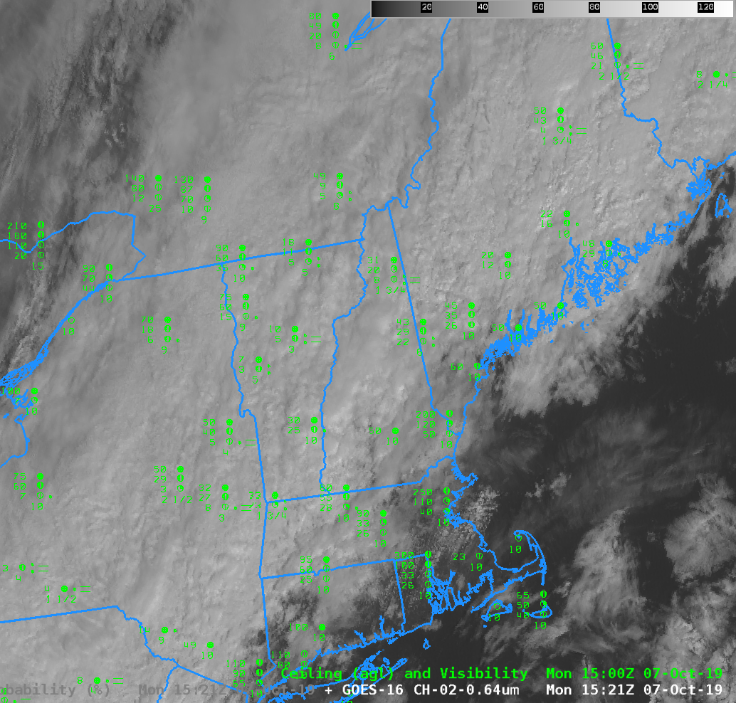
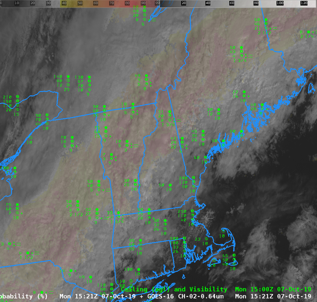
GOES-16 ABI Band 2 (0.64 µm) from 0902-1312 UTC on 9 May 2018 (Click to enlarge)

GOES-16 Visible Imagery on the morning of 9 May 2018 shows the steady erosion of fog in/around the Bay of Fundy, and along coastal Maine.  The default 5-minute temporal cadence with the CONUS GOES-16 sector allows for a precise observation for when coastal fog will clear.

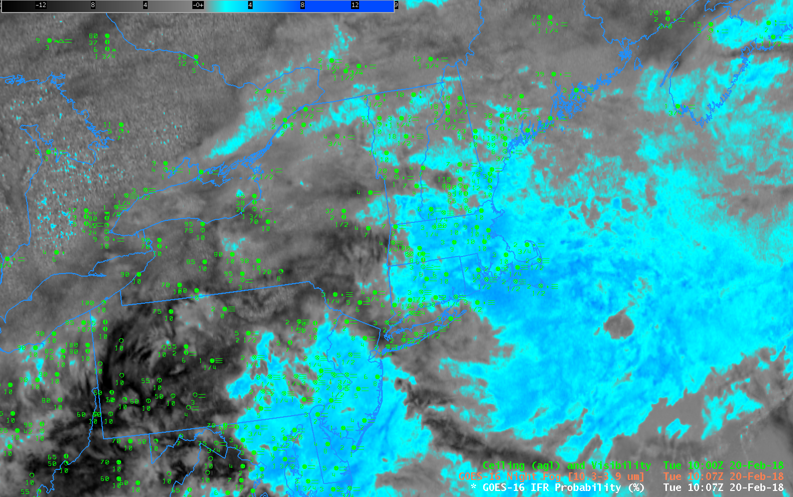
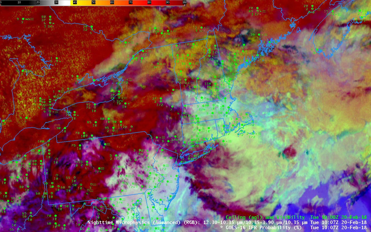
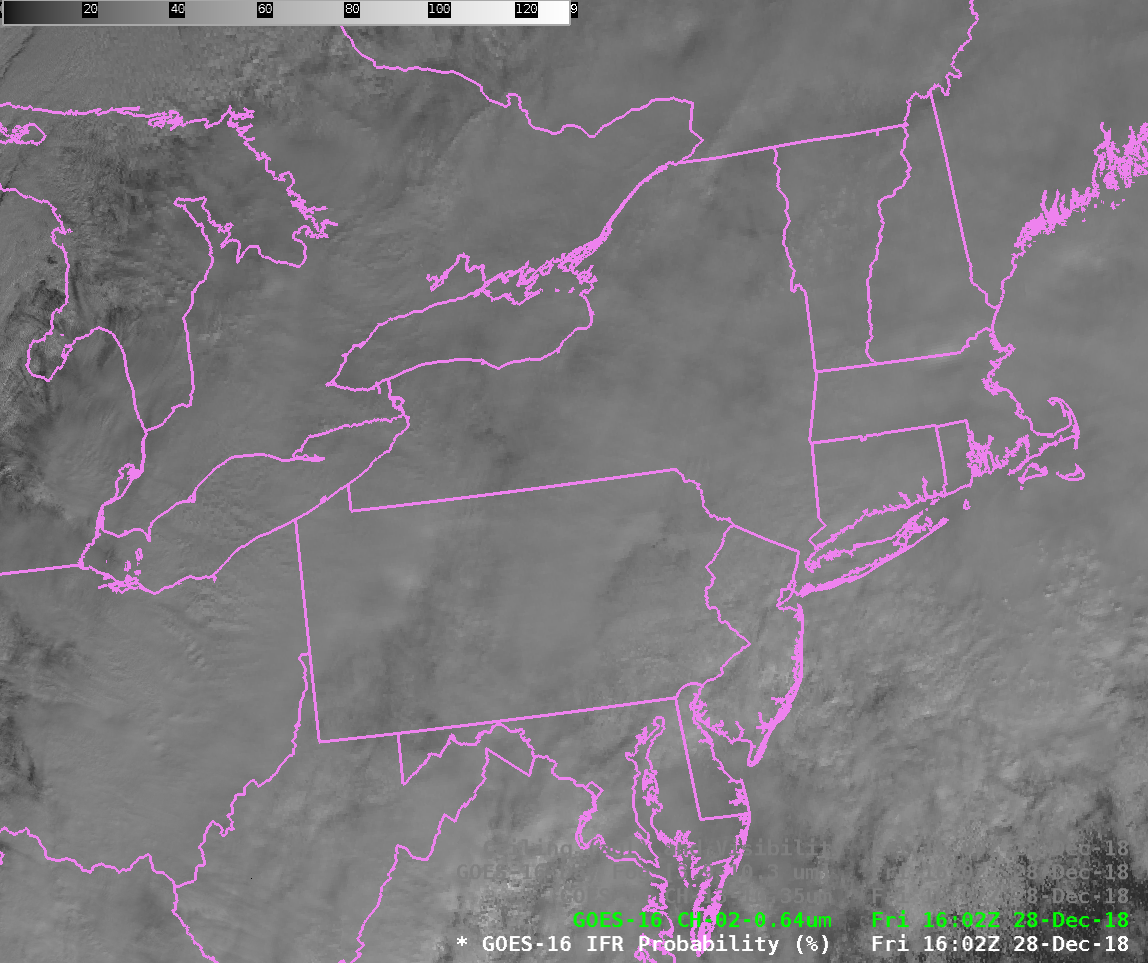
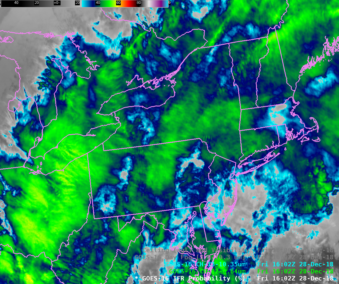
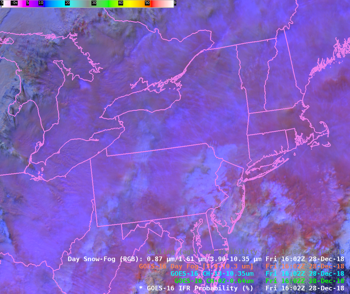
The satellite view of the fog in the bay was unobstructed by high clouds.  (except to the east of Nova Scotia, where a cirrus shield is apparent in the visible animation above, and in animation below)    Thus, the GOES-16 Night Fog Brightness Temperature Difference field (10.3 µm- 3.9 µm), below, could ably capture the fog’s presence and evolution.  The animation of that product, below, shows how the signal changes at sunrise as reflected solar 3.9 µm radiation overwhelms the brightness temperature difference (driven at night by differences in emissivity at 3.9 and 10.3 µm from cloud droplets): the sign flips.  Because the fog was captured in the Night Fog Brightness Temperature Difference, it was also present in the Nighttime Microsphysics RGB Composite (here), although the color associated with fog  changes as the sun rises, and clear skies also allowed the Day Snow Fog RGB Product to show the fog during the day (here).

None of the Satellite-based products can provide information on the likelihood of fog over the ocean to the east of Nova Scotia, however, because the presence of cirrus clouds there prevents the satellite from viewing low clouds.  What products can help with that?

GOES-16 ABI Night Fog Brightness Temperature Difference (10.3 µm – 3.9 µm) from 0817-1312 UTC on 9 May 2018 (Click to enlarge)

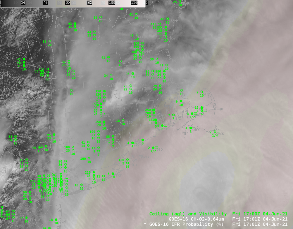
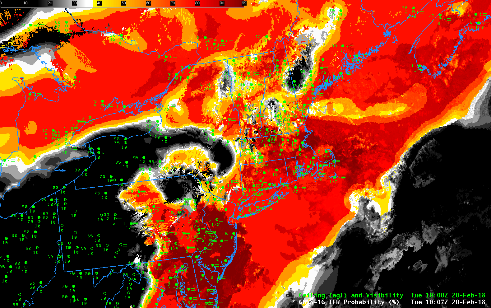
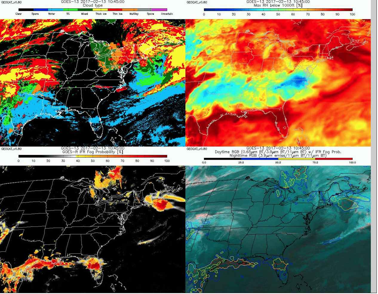
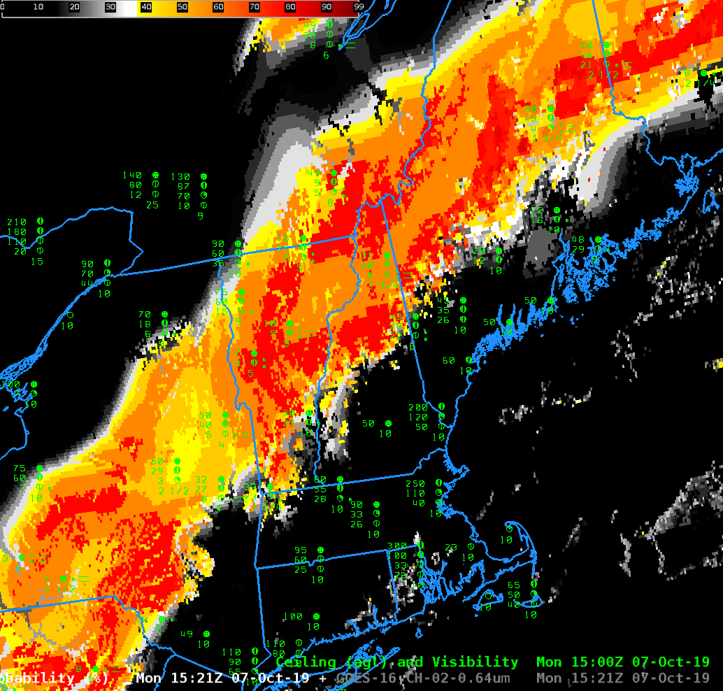
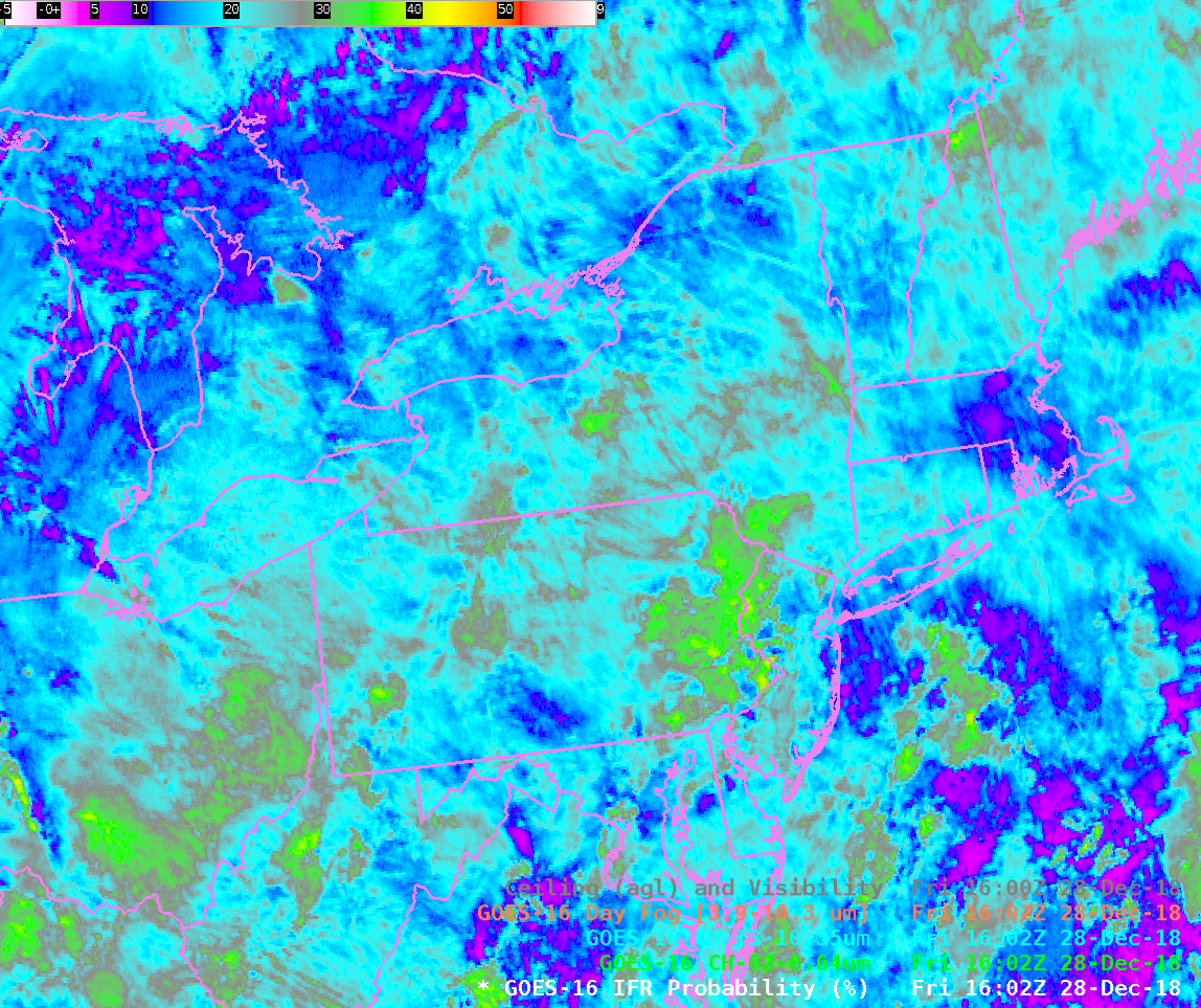
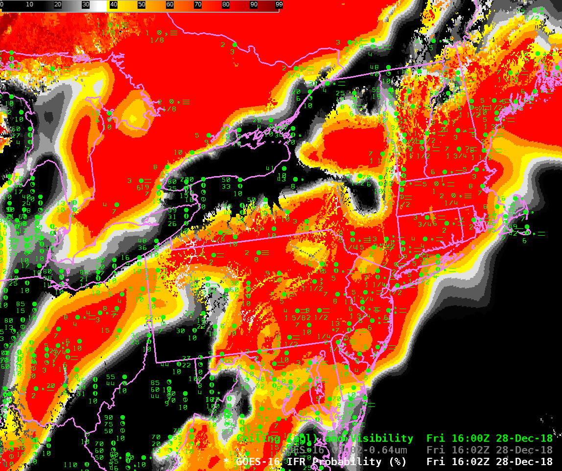
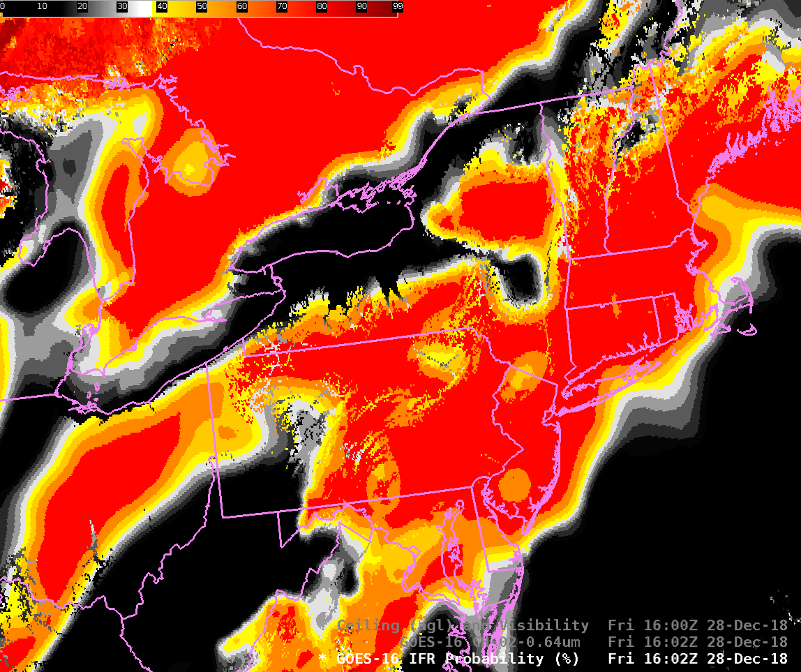
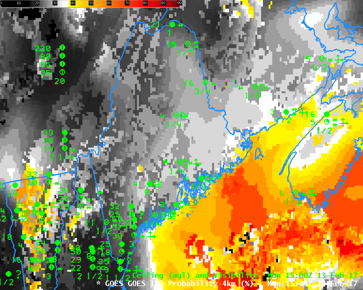
GOES-16 IFR Probability fields, below, combine together satellite and model information to determine where IFR Conditions are most likely.  Very high probabilities exist where other satellite fog detection products suggest the presence of fog/low stratus (and where surface observations confirm the presence of fog).  But there are also high probabilities over the ocean east of Nova Scotia where satellite-only fog detection fails because of the presence of high clouds;  this large signal is derived from Rapid Refresh data there that suggests low-level saturation. IFR Probability combines the strengths of both satellite data and model output to provide useful information to a forecaster.

GOES-16 IFR Probability (10.3 µm – 3.9 µm) from 0817-1322 UTC on 9 May 2018

(Thanks to Paul Ford, ECC Canada, for alerting us to this event)

Added: The GOES-16 ABI Band 3 (0.86 µm) “Veggie” Band, which has great land/sea contrast, shows the fog encroaching into the Bay of Fundy during the day on 8 May. Note in particular how the low clouds race up the west coast of Nova Scotia near sunset.

GOES-16 ABI Band 3 (0.86 µm) from 1512-2257 UTC on 8 May 2018 (Click to enlarge)

IFR Conditions in the Northeast

GOES-16 IFR Probability, 1007 UTC on 20 February 2018, along with surface observations of ceilings and visibilities (Click to enlarge)

A complex set of Low Pressure systems over the eastern half of the United States brought multiple cloud layers and IFR conditions to the northeastern United States on 20 February. The image above shows the IFR Probability field at 1007 UTC. IFR Conditions are apparent from the Chesapeake Bay northeastward through southeastern Pennsylvania and New York and coastal New England, as well as over southeastern Ontario Province in Canada and the Canadian Maritimes. These are also regions where IFR Probabilities are high, generally exceeding 80%. In regions where IFR conditions are not observed (Western Pennsylvania and Ohio, for example), IFR Probabilities are generally small.

When multiple cloud decks are present, as occurred on 20 February, satellite-only detection of low clouds is a challenge, as shown with by the brightness temperature difference field (10.3 µm – 3.9 µm), called the ‘Night Fog’ difference in AWIPS, below. High and mid-level clouds (grey/black in the enhancement used) make satellite detection of low-level stratus impossible.  So, for example, stations with IFR conditions over Long Island sit under a much different enhancement in the brightness temperature difference field compared to stations with IFR conditions over southern New Jersey and southeastern Pennsylvania.

Because the Brightness Temperature Field cannot view the low clouds, the Nighttime Microphysics RGB (shown below the Brightness Temperature Difference field) similarly cannot identify all regions of low, warm clouds — typically yellow or cyan in that RGB.

Night Fog Brightness Temperature Difference field (10.3 µm – 3.9 µm) at 1007 UTC on 20 February 2018, along with surface observations of ceilings and visibilities (Click to enlarge)

NightTime Microphysics RGB at 1007 UTC on 20 February 2018, along with surface observations of ceilings and visibilities (Click to enlarge)

IFR Probabilities with a strong storm in Maine

GOES-R IFR Probabilities, 0100-1000 UTC on 7 April 2017, along with surface reports of ceilings and visibilities (Click to enlarge)

Note:  GOES-R IFR Probabilities are computed using Legacy GOES (GOES-13 and GOES-15) and Rapid Refresh model information;  GOES-16 data will be incorporated into the IFR Probability algorithm in late 2017

A strong storm over the northeastern United States produced widespread IFR conditions over that region.  The storm was also accompanied by multiple cloud layers, however, and that made diagnosis of regions low clouds/fog difficult.  For these cases, a fused data approach is vital — using model information (in the case of IFR Probability, above, the model is the Rapid Refresh) to provide information at low levels allows for a better tool to alert a forecaster to the presence of reduced visibilities.

In the animation above, Maine intially shows IFR Probabilities around 50% — but the flat nature of the field should alert a user to the fact that satellite predictors cannot be included in the computation of IFR Probabilities because high clouds are preventing a satellite view of low clouds.  Accordingly, the computed Probability is lower.  In contrast, high clouds are not present over southern New England at the start of the animation, and IFR Probabilities are much larger there:  both satellite and model predictors are used. As the high clouds lift north from northern New England the region of higher IFR Probabilities expands from the south.

Note the influence of topographic features on the IFR Probability field.  The Adirondack Mountains and St. Lawrence Seaway have higher and lower Probabilities, respectively, because of the higher terrain in the Mountains, and the lower terrain along the St. Lawrence.

An example of why fused data are important is shown below.  Look at the conditions in Charlottetown, on Prince Edward Island, in the far northeast part of the domain.  Between 0315 and 0400, ceilings and visibilities deteriorate as IFR Probabilities increase.  The brightness temperature difference field, at bottom, shows no distinct difference between those two times because the clouds being viewed are high clouds.

IFR Conditions over Maine

GOES-R IFR Probability and with surface observations of ceilings and visibilities, 1045 UTC on 13 February 2017 (Click to enlarge)

A strong storm off the East Coast of the United States produced a variety of winter weather over Maine on 13 February 2017, including Blizzard conditions. Although ceilings and visibilities above show IFR or near-IFR conditions at 1045 UTC, GOES-R IFR probabilities over Maine are small (less than 20%). Why?

The image below from this site shows Cloud Type, Low-Level Saturation, IFR Probability, and the Nighttime Microphysics.  Both Ice clouds and falling snow are widespread over Maine. GOES-R IFR Probabilities typically assume saturation with respect to water.   The Gray, ME morning sounding shows maximum RH (with respect to water) at only 94% (Link).  Assuming saturation with respect to water rather than with respect to ice may be a source of error that will have to be investigated in the future.

Note that after sunrise, IFR Probabilities increased over Maine to values between 30 and 45% (Link).

Satellite-derived Cloud Type (upper left), Maximum Low-Level Relative Humidity in the Rapid Refresh (upper right), GOES-R IFR Probability (lower left) and Nighttime microphysics (lower right), all from 1045 UTC on 13 February (Click to enlarge)

IFR Conditions over Maine

GOESR_IFR_0500_1215_12June2016anim

GOES-R IFR Probability, and surface plots of ceilings and visibility, 0500-1215 UTC on 12 June 2016 (Click to enlarge)

IFR Probability fields, above (a slower animation is here), show high probabilities of IFR Conditions over much of Maine, but a definite western edge is also present, moving eastward through New Hampshire and Vermont and reaching western Maine by 1215 UTC. The screen capture below, from this site, shows IFR (station models with red) and Low IFR Conditions (station models with magenta) over much of southern Maine at 1200 UTC on 12 June in advance of a warm front.

Careful inspection of the IFR Probability animation shows a field at 1000 UTC that is very speckled/pixelated. This likely results from cloud shadowing. The combination of a very low sun and multiple cloud layers resulted in many dark regions in the visible imagery that the cloud masking may have interpreted as clear regions. (Click here for a toggle between Visible Imagery and GOES-R IFR Probabilities at 1000 UTC).

MetarPLOT_1200UTC

Surface plot at 1200 UTC 12 June 2016. See text for details (Click to enlarge)

Low IFR Probability fields are also computed by the GOES-R Algorithms. Values are typically smaller than IFR Probability. Plots of Low IFR and IFR Probabilities at 0700 and 1215 UTC are shown below.

GOESR_IFR_LIFR_0700_1215_12June2016toggle

GOES-R Low IFR Probability and GOES-R IFR Probability, 0700 and 1215 UTC (Click to enlarge)

IFR Conditions with a Coastal Storm

GOES_IFRPanim_0400_1515_05Feb2016

GOES-R IFR Probabilities, hourly from 0400 through 1515 UTC, 5 February 2016 (Click to enlarge)

IFR Conditions frequently occur with storms along the East Coast. Satellite detection of such conditions is very difficult because of the multiple cloud layers that accompany cyclogenesis. The IFR Probabilities, above, have a character that reflects their determination solely from Rapid Refresh Data. That is, Satellite Predictors were not considered over much of New England because of the presence of multiple cloud layers, as suggested in the Water Vapor animation below.

IFR Probability fields are initially entirely offshore in the animation above, and IFR conditions are not observed over southern New England.  Note how IFR probabilities initially increase over land over southern New Jersey and then quickly move northeastward into southern New England as IFR Conditions develop.  Because satellite predictors are unavailable in these regions (on account of the many clouds layers), the simultaneous development of high IFR Probabilities with observed IFR Conditions argues for a good simulation of the observed weather by the Rapid Refresh.  Fused data products such as IFR Probability fields join the strengths of different systems to provide a statistically more robust field than is possible from the individual pieces.

When daytime arrives — at around 1215 UTC in the animation above — a distinct transition is apparent in the GOES-R IFR Probability fields.  This occurs because Satellite Data — visible satellite data — can be used during daytime to articulate the regions of cloudiness with more precision.  Because cloudiness in general is better defined, IFR Probability fields (that require the presence of clouds) increase somewhat, and the color table used emphasizes that change.

WV__0400_1300_05Feb2016anim

GOES-13 Water Vapor 3-hourly Animation, 0400-1300 UTC, 5 February 2016 (Click to enlarge)