Monthly Archives: February 2015

When IFR Probability Fields are stationary

GOES_IFR_PROB_20150217

GOES-R IFR Probability Fields computed from GOES-13 on 17 February 2015, times as indicated (Click to enlarge)

Different kinds of fields are used in the computation of IFR Probability fields: fields that can change quickly with time (Satellite observations of brightness temperature difference, satellite observations of cloud type, model output showing low-level moisture); fields that can change slowly with time (Sea surface temperature and surface emissivity fields), and fields that don’t change (Topography). An IFR Probability field that is relatively constant with time, then, as over northern Alabama in the animation above, is showing the effects of terrain (color shaded in the image below). In this case, higher terrain is on either side of the Tennessee River Valley in northern Alabama is apparent in the IFR Probability fields (Lowered ceilings are more likely over the higher terrain than over the adjacent, lower river valley). Transitory patterns associated with propagating weather features are also apparent.

GOES_IFR_PROB_20150217_1145

Topography over northern Alabama and surrounding states (Click to enlarge)

Fog Development on the Texas Gulf Coast

GOES_IFR_BTD_20150211_0200

GOES-R IFR Probabilities and GOES-East Brightness Temperature Difference fields (10.7µm – 3.9µm) at 0200 UTC on 11 February 2015 (Click to enlarge)

GOES_IFR_BTD_20150211_0315

GOES-R IFR Probabilities and GOES-East Brightness Temperature Difference fields (10.7µm – 3.9µm) at 0315 UTC on 11 February 2015 (Click to enlarge)

Dense fog developed along the Texas Gulf Coast late on 10 February and early on 11 February. GOES-R IFR Probabilities gave an advance warning of the fog development, as shown above. Toggles between the GOES-R IFR Probability and the Brightness Temperature Difference Product (a heritage method of fog detection) show a IFR Probability signal at 0200 UTC; that signal steadily increased until 0315 UTC when a signal started to become apparent in the Brightness Temperature Difference Field. In this case, IFR Probabilities gave extra lead time to alert the forecaster to the development of fog. (This has happened before) Note also how the IFR Probability fields screen out false positive signals of fog over West Texas.

Hourly animations for GOES-R IFR Probability and GOES-13 Brightness Temperature Difference fields are below. The IFR Probability fields neatly overlap regions with IFR or near-IFR conditions. Note the impact of the high clouds that move over coastal south Texas after 1200 UTC; the brightness temperature difference field and the GOES-R IFR Probability fields both are affected.

GOES_IFR_PROB_20150211_02_13

GOES-R IFR Probability hourly from 0200 through 1300 UTC 11 February 2015 (Click to enlarge)

US_11-3.9_Sat_20150211_02_13

GOES-13 Brightness Temperature Difference (10.7µm – 3.9µm) hourly from 0200 through 1300 UTC 11 February 2015 (Click to enlarge)

Fog in the Pecos River valley of New Mexico

GOES_IFR_PROB_20150206_0700_1300

GOES-R IFR Probabilities computed from GOES-13 and Rapid Refresh Data, 0700-1300 UTC, 6 February 2015 (Click to enlarge)

Fog developed over the Pecos River valley in southeastern New Mexico early on the morning of 6 February. This small-scale feature was captured well by the GOES-R IFR Probability fields, shown above. Probabilities increased quickly between 0745 and 0800 UTC. In contrast, the brightness temperature difference product, below, showed little signal until around 1000 UTC. GOES-R IFR Probability fields responded more quickly to the possible development of fog and in this case could have alerted any forecaster to its imminent formation. IFR conditions were present at Carlsbad (KCNM), Artesia (KATS) and Roswell (KROW) by 1100 UTC.

US_11-3.9_Sat_20150206_0700_1300

GOES-13 Brightness Temperature Difference fields, 0700 through 1300 UTC, 6 February 2015 (Click to enlarge)

MODIS data from Terra and Aqua, and VIIRS data from Suomi NPP give occasional snapshots (at high resolution) of conditions. Terra (just before 0500 UTC) and Aqua (around 0900 UTC) data were used to compute IFR Probabilities, and the high resolution data, below, is consistent with the development of fog over night. The 0900 UTC image especially suggests the possibility of fog.

MODIS_IFR_PROB_20150206_0448_0901

MODIS IFR Probability from Terra (0448 UTC) and Aqua (0901) UTC on 6 February 2015 (Click to enlarge)

Suomi NPP data are not yet used to compute IFR Probabilities. The toggle, below, of the Day Night Band and the Brightness Temperature Difference at 0835 UTC does not show convincing evidence of fog at that time. The Day Night Band is very crisp because of the near Full Moon that provided ample lunar illumination.

VIIRS_DNB_FOG_20150206_0835

Suomi NPP Day Night Band and Brightness Temperature Difference, 0835 UTC, 6 February 2015 (Click to enlarge)

The imagery above all suggest that the presence of model data — from the Rapid Refresh — enhanced the satellite data as far as suggesting IFR conditions.

South Texas Fog and low stratus

GOES_IFR_PROB_20150204anim

GOES-R IFR Probabilities, half-hourly from 0045 UTC to 1215 UTC on 4 February 2015, along wtih surface reports of ceilings and visibilities (Click to enlarge)

Fog developed over south Texas during the morning of 4 February. How did the GOES-R IFR Probability Products perform for this example, and what can be learned from them? There are at least two distinct regions in the animation above. Over much of southeast Texas, the IFR Probability field suggests multiple cloud layers are present. IFR Probabilities are smaller here because satellite-based cloud information cannot be used in the algorithm in regions where high/mid-level clouds preclude a satellite’s view of low stratus and fog. It is important to interpret the IFR Probability fields with knowledge of the cloud levels that are present. Towards the middle of the loop, fog develops in/around Midland over the high Plains. IFR Probabilities are large there because satellite data are used as a predictor because high clouds are not impeding the satellite’s view of the developing region of fog/stratus. Brightness Temperature Difference Fields from GOES, below, show the difficulty in using that field to detect fog/low stratus in regions where multiple cloud layers exist. There are many stations underneath high clouds that have undetectable (via satellite) IFR conditions.

US_11-3.9_Sat_20150204_0140_1215

GOES-13 Brightness Temperature Difference (10.7µm – 3.9µm), 0245 – 1215 UTC 4 February 2015 (Click to enlarge)


MODIS_GOES_IFRPROB_20150204_0915

Toggle between GOES-based and MODIS-based IFR Probabilities at 0915 UTC on 4 February 2015 (Click to enlarge)

MODIS data from Aqua can also be used to compute IFR Probabilities, as shown above. In general, there is very good agreement between GOES and MODIS-based fields, but there are some very interesting differences along the limb of the MODIS scan in central TX where GOES data shows smaller values of IFR Probabilities than is shown in the MODIS fields — for example at San Angelo (KSJT), Kirksville (KCOM) and Brady (KBBD). This occurs in a region where limited observations show near-IFR conditions. The higher values along the limb of the MODIS scan are likely due to limb brightening that arises because the radiation being detected comes from a path that traverses more of the (colder) upper atmosphere. The affect is wavelength-dependent, and thus will show up in a brightness temperature difference field as a stronger signal, and that stronger signal will influence the IFR Probability fields. In short: interpret MODIS IFR Probability fields along the edge of the MODIS swath with this knowledge of limb effects.

VIIRS_FOG_20150204_0279_0910

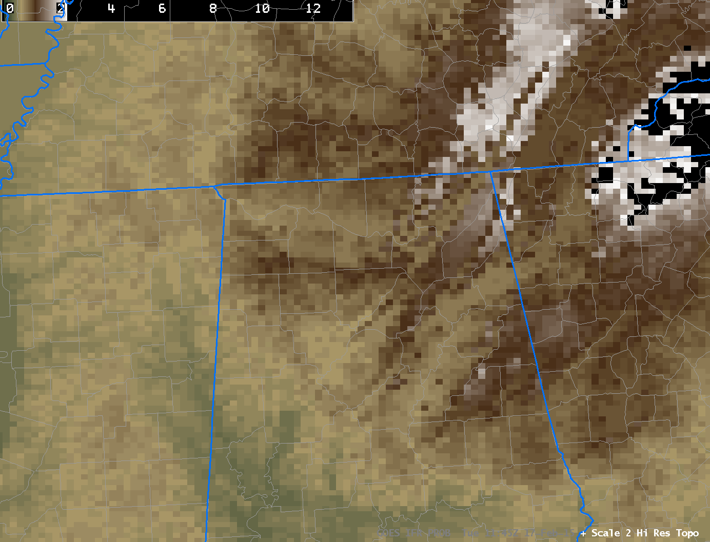
Brightness Temperature Difference (11.35 µm – 3.74 µm) from Suomi NPP at 0729 and 0910 UTC (Click to enlarge)

Suomi NPP also viewed the evolving fog/stratus field over Texas, and two brightness temperature difference fields, from sequential overpasses, are shown above. Brightness Temperature Difference fields can only give information about the top of the cloud, not the cloud base, and the cloud base is the important piece of information needed for fog detection. There are regions under the high clouds, for example, with IFR conditions. The eye is drawn by the enhancement to regions of low clouds/stratus, but important visibility restrictions are occurring elsewhere as well. The high resolution imagery of Suomi NPP does show compelling structures in the cloud fields, however. Note also the presence of limb brightening: Compare the brightness temperature fields west of Midland during the two times.

The Day Night Band from the morning of 4 February — near Full Moon — showed excellent structure in the cloud features, all made visible by ample lunar illumination as shown below. It is difficult, however, to use cloud-top information from the Day Night band to infer the presence of IFR conditions.

VIIRS_DNB__REF_20150204_0729_0910

Day Night Band (0/70 µm) from Suomi NPP at 0729 and 0910 UTC (Click to enlarge)