Category Archives: Pacific Northwest

IFR Probability for situational awareness over the Pacific Northwest

GOES-17 IFR Probability fields, 1011-1321 UTC on 10 December 2021; Surface observations of ceilings (above ground level) and visibility are also included (Click to enlarge)

The animation above shows GOES-17 IFR Probabilities over the Pacific Northwest. This is a good situational awareness tool for fog/low stratus because it highlights regions where IFR conditions are most likely. That is, it is a quantitative product. The product also has knowledge of terrain height; if low clouds exist in regions where terrain might be rising into the clouds (for example to the northeast of Seattle WA, and to the east of Portland OR, and in Olympic National Park), IFR probabilities are heightened (pun not really intended).

The Nighttime microphysics RGB, shown below, can also be used for qualitative situational awareness. In this case, the region of low clouds over western Washington, around Spokane (where observations show IFR conditions) and to the north, is highlighted as expected (the yellow color that is structured so that individual valleys are obvious). IFR Probabilities north of Spokane are not large, however, suggesting that model simulations there (from the Rapid Refresh model) do not show low-level saturation. (Observations at KOMK — Omak Washington — show near-IFR conditions). Another strength of IFR Probability is that it supplements satellite data where the satellite cannot view low clouds. High clouds to the east of Seattle and Portland are obscuring the view of low clouds in that region where IFR Probabilities are large and where ceilings and visibilities are likely reduced.

GOES-17 Nighttime Microphysics RGB (PACUS sector), 1011 – 1321 UTC on 10 December 2021 (Click to enlarge)

Fog in Oregon’s Willamette Valley

GOES-16 IFR Probability, 1451 UTC on 2 November 2020 along with 1500 UTC observations of ceilings and surface visibility (Click to enlarge)

GOES-16 IFR Probability fields, above, show very high IFR Probability values over the Willamette Valley of Oregon to the south of Portland; surface observations in the region show IFR conditions from Salem (KSLE) southward through Eugene (KEUG) to Roseburg (KRBG). IFR Probability is also large along the coast, with IFR conditions reported at Newport (KONP) and North Bend (KOTH). The 10.3 µm – 3.9 µm “Night Fog” Brightness Temperature Difference field, below, also has a modest signal in the Valley, and along the coast, giving a qualitative (but not quantitative) estimate of fog.

GOES-16 Night Fog Brightness Temperature Difference (10.3 µm – 3.9 µm) at 1451 UTC on 2 November 2020 (Click to enlarge)
GOES-16 Cloud Thickness (“Fog Depth”) from 1451-1506 UTC on 2 November 2020 (Click to enlarge)

GOES-R Cloud Thickness (labeled as Fog Depth in TOWR-S Build 19) can be used to estimate radiation fog dissipation time. Values are not computed during the time of rapidly-changing reflected solar radiance (i.e., for the times around sunrise and sunset); the last pre-sunrise value can be used in concert with this scatterplot to estimate burn-off times. Values at 1451 UTC in the Willamette valley peak at around 380 m. This suggests a burn-off time (if this is radiation fog and not advection fog) of about two hours according to the scatterplot below, i.e., shortly before 1700 UTC.

Scatterplot: Last pre-sunrise Cloud Thickness value vs. Dissipation Time. (Click to enlarge)

Visible imagery, below, at 1601 and 1706 UTC do show a trend towards clearing. The scatterplot can underestimate clearing time if (1) the sun angle is lower than at the points used to create the scatterplot or (2) if the fog is not strictly a radiation fog. In either event, however, the values from day to day should give useful information. For example, if today’s last pre-sunrise cloud thickness is greater than yesterday’s, then the burn-off time today should be later than yesterday.

GOES-16 Visible (0.64) Imagery and surface observations of ceilings/visibility at 1601 and 1706 UTC on 2 November 2020 (click to enlarge)
GOES-16 Visible (0.64) Imagery and surface observations of ceilings/visibility at 1901 UTC on 2 November 2020 (click to enlarge)

Fog/low stratus dissipated shortly after the 1901 UTC image shown above.

How to tell at a glance that IFR Probability is model-driven: Pacific Northwest version

GOES-16 IFR Probability at 10-minute timesteps, 1051 to 1721 UTC on 6 February 2020 (Right click to enlarge)

The animation above, of GOES-16 IFR Probability, shows high IFR values in regions over western Washington and Oregon, and those high values correlate spatially very well with surface observations of low ceilings and reduced visibilities.b You will note a couple things in the animation: The field is mostly stationary, with slight adjustments on every hour. Those small changes reflect the change in the model fields (hourly Rapid Refresh) that are used to complement satellite estimates of low clouds in the computation of IFR Probabilities.

On this day, the satellite did not view many low clouds (some are apparent in southwestern Oregon). The flat field (vs. the more pixelated view over southwest OR, and also occasionally in the west-northwest flow coming in off the Pacific) suggests only model data are being used. The stepwise changes on the hour also suggest that.

The animation of the Night Fog Brightness Temperature Difference (10.3 µm – 3.9 µm) field, below, has a signal that is consistent with the lack of observed stratus over the coastal Pacific Northwest. Note also how the Night Fog Brightness temperature difference field flips sign as the Sun comes up and the 3.9 µm signal becomes larger due to reflected solar radiance with a wavelength of 3.9 µm.

GOES-16 Night Fog Brightness Temperature Difference (10.3 µm – 3.9 µm) at 10-minute timesteps, 1051 to 1721 UTC on 6 February 2020 (Right click to enlarge)

GOES-16 views of the Pacific Northwest show fairly large pixel sizes. NOAA/CIMSS scientists have been creating GOES-17 IFR Probability for the past couple weeks, and this product will become available via an LDM field in the near future.

Note that GOES-17 IFR Probability products are available online at https://cimss.ssec.wisc.edu/geocat.

Fog Detection when Cirrus is present

GOES-16 NightTime Microphysics, Night Fog Brightness Temperature Difference (10.3 µm – 3.9 µm) and IFR Probability at 1206 UTC on 4 November 2019, along with 1200 UTC observations of ceilings and visibilities (Click to enlarge)

Fog can be a challenge to detect from satellite for two reasons: High clouds can block the satellite’s view of low clouds, or low clouds (stratus) can be detected but the satellite cannot accurately determine the cloud base. The toggle above cycles between the Night Fog Brightness Temperature difference (10.3 µm – 3.9 µm), the Nighttime Microphysics RGB (the Night Fog Brightness Temperature Difference is the green component of that RGB), and GOES-R IFR Probability.

The Night Fog Brightness Temperature Difference can be used to detect low stratus clouds because the small water droplets that make up those clouds have different emissivities at 10.3 µm and 3.9 µm: water droplets do not emit 3.9 µm radiation as a blackbody would, but they do emit 10.3 µm radiation more nearly like a blackbody. Thus the amount of energy at 3.9 µm collected by the satellite is smaller than it would be above a blackbody emitter. The computation of the blackbody temperature associated with the collected energy assumes a blackbody emission. Because that’s not the case at all wavelengths above clouds made of water droplets, 3.9 µm brightness temperatures are colder than those computed from observed 10.3 µm energy.

The Night Fog brightness temperature difference field allows an observer to infer the presence of low clouds over the Pacific Ocean, in and around Portland OR on the Columbia River to the ocean, and also northward towards Puget Sound, and in the Willamette Valley between Portland and Eugene OR. There is also a signal over north-central Oregon that is likely unrelated to clouds — variable surface soil emissivity in that region is affecting this brightness temperature difference (The GOES-R Cloud Phase product and Cloud Mask both show no cloud signal in that region).

Note that a cirrus shield is apparent over the northeast half of the image. The cirrus covers most of Puget Sound in Washington, and the Brightness Temperature Difference field can therefore not give information about low clouds (except where breaks in the cirrus occur — such as in the Strait of Juan de Fuca).

The Nighttime Microphysics RGB is a way to identify low clouds — but its information is coming from the Night Fog brightness temperature difference and it has limitations that are similar to those with the brightness temperature difference, namely: what is going on under cirrus clouds, and how close to the ground are the low clouds that are detected? In the RGB, low clouds will have a yellowish hue (red — the split window difference and green — the night fog brightness temperature difference — make yellow). The RGB shows different values over Portland than over the Willamette Valley because the clouds are warmer over Portland (as detected by the clean window 10.3 as the blue part of the RGB) and the split window difference field (the red part of the RGB) shows larger values over the Willamette Valley.

IFR Probability shows a a strong and consistent signal from Portland south to Eugene, and also over the Pacific, and north of Portland into the southern Puget Sound. In these regions, Rapid Refresh Model data are showing the presence of low-level saturation, a good indicator that IFR conditions may be present. IFR Probability shows small values under the region of low clouds detected by satellite over the Strait of Juan de Fuca; the Rapid Refresh model there is not showing low-level saturation. There is also a small signal in the clear skies over north-central Oregon where a brightness temperature difference is occurring because of soil-driven emissivity differences.

Use IFR Probability to ascertain the likelihood of fog underneath cirrus decks, or to determined the likelihood of stratus decks reaching the surface (that is, if stratus is actually fog).

Fog over the Pacific Northwest: Where is it?

GOES-17 imagery in this blog post is made from GOES-17 Data that are preliminary and non-operational!

Night Time Fog Brightness Temperature Difference (10.3 µm – 3.9 µm) from GOES-16 and (preliminary, non-operational) GOES-17, 1202 UTC on 3 December 2018 (Click to enlarge)

The toggle above shows GOES-16 and GOES-17 Night Fog Brightness Temperature difference fields over the Pacific Northwest shortly after 1200 UTC on 3 December 2018.  The Pacific NW is a lot farther from the sub-satellite point (nadir) of GOES-16 (75.2 West Longitude) than from the sub-satellite point (nadir) of GOES-17 (at 137.2 W Longitude).  Thus, the GOES-16 view is has inferior spatial resolution.  There are also different parallax shifts for clouds between the two views.  The scene includes plenty of stratus, based on the observations, and isolated pockets of IFR conditions:  Spokane WA, Stampede Pass, WA, Pendleton OR, Medford OR, Salem OR.  It’s difficult to tell at a glance from the Brightness Temperature Difference field where the lowest ceilings and poorest visibilities are — because the satellite sees the top of the cloud, and it’s difficult to infer cloud base properties from infrared imagery of the cloud top.

The Advanced Nighttime Microphysics RGB can also be used to detect low ceilings, because its green component is the Night Fog Brightness Temperature Difference as shown above.  The toggle below compares the GOES-16 and GOES-17 RGBs.  Again, it is difficult to pinpoint at a glance where the IFR conditions are occurring in this product.

There are subtle differences in the colors of the RGB from the two satellites.  These are related to the distance from the sub-satellite point.  Limb cooling will cause the brightness temperatures from the GOES-16 Clean Window to be slightly cooler than the GOES-17 values, and that will affect the color:  The Clean Window is the Blue component of the RGB.  In addition, the Split Window Difference values will be slightly different because of the different amounts of limb cooling in 12.3 µm and 10.3 µm brightness temperatures.  GOES-17 data also includes striping that is being addressed with ongoing calibration work with the satellite.

Advanced Nighttime Microphysics RGB from GOES-16 and GOES-17 at 1202 UTC on 3 December 2018 (Click to enlarge)

The toggle below shows, (from GOES-16 data) the 10.3 µm – 3.9 µm Brightness Temperature Difference, the Nighttime Microphysics RGB, and the IFR Probability fields at 1202 UTC. IFR Probability fields include information about low-level saturation from the Rapid Refresh model, and that information allows the product to screen out regions of mid-level stratus; thus, the region of IFR conditions is better captured.  There are three main regions:  eastern WA southwestward to Pendleton OR, Seattle southward into Oregon, and the peaks of central Washington.

GOES-16 Night Fog Brightness Temperature Difference (10.3 µm – 3.9 µm), Nighttime Microphysics RGB and IFR Probability, 1202 UTC on 3 December 2018 (Click to enlarge)

Fog under multiple cloud layers

GOES-16 Night Fog Brightness Temperature Difference (10.3 µm – 3.9 µm), 1137 – 1452 UTC on 31 October 2018 (Click to animate)

Consider the imagery above: The Night Fog Brightness Temperature Difference (10.3 µm – 3.9 µm) product can be used to highlight regions of low clouds (cloud made up of water droplets) because those water droplets do not emit 3.9 µm radiation as a blackbody (but do emit 10.3 µm radiation nearly as a blackbody), and the conversion of sensed radiance to brightness temperature assumes blackbody emissions. Thus, the 10.3 µm brightness temperature is warmer than at 3.9 µm. In the enhancement used, low stratus clouds are shades of cyan. Is there fog/low stratus along the coast of the Pacific Northwest? How far inland does it penetrate. It is impossible in this case (and many similar cases) to tell from satellite imagery alone because multiple cloud layers associated with a storm moving onshore prevent the satellite from seeing low clouds. The animation shows the Brightness Temperature Difference field along with surface reports of visibility and ceilings.  IFR and near-IFR conditions are widespread, but there is little correlation between their location and the satellite-only signal.

GOES-16 Night Fog Brightness Temperature Difference (10.3 µm – 3.9 µm), 1137 – 1452 UTC on 31 October 2018, along with surface reports of ceilings (AGL) and visibility (Click to animate)

GOES-R IFR Probability fields fuse together satellite information and model data to provide a better estimate of where IFR conditions might be occurring. The animation below, for the same times as above, shows a high likelihood of IFR conditions (as observed) over much of the eastern third of Washington State. The satellite doesn’t give information about the near-surface conditions in this case, but the Rapid Refresh data strongly suggests low-level saturation, so IFR probabilities are high. The field also correctly shows small likelihood of IFR probailities over coastal southern Oregon and northern California. The Rapid Refresh data used have 13-km resolution, however; fog at scales smaller than that may be present — in small valleys for example.

GOES-16 IFR Probabilities, 1137 – 1452 UTC on 31 October 2018 (Click to animate)

Detecting Fog under a Pall of Smoke in the Pacific Northwest

HRRR forecast of Vertically-Integrated Smoke over the Pacific Northwest (for more information see text), forecast valid at 1200 UTC on 30 July 2018 (Click to enlarge)

When smoke covers a geographic region, visible detection of low-level fog is difficult because smoke can scatter or obscure the signal from the low-level clouds.  The image above shows a Vertically Integrated Smoke Forecast from a High-Resolution Rapid Refresh Model simulation in Real Earth (link). Thick smoke was predicted to occur over the coast of Oregon.

The animation below steps through the GOES-R IFR Probability, and then the ‘Blue Band’ (0.47 µm), the ‘Red Band’) (0.64 µm), the ABI channel with the highest spatial resolution, the ‘Veggie Band’ (0.86 µm) and the ‘Snow/Ice Band’ (1.61 µm). Two things of note: Because of the low sun angle, and the enhanced forward-scattering properties of smoke at low sun angle, it is very hard to detect fog through the smoke in the visible wavelengths near Sunrise. As the wavelength of the observation increases, scattering is less of an issue. In addition, smoke is more transparent to longer wavelength radiation. Thus, the cloud edges become more apparent under the smoke in the 0.86 µm and especially the 1.61 µm imagery compared to the visible.

GOES-16 IFR Probability, and GOES-16 Single Bands (Band 1, 0.47 µm, Band 2, 0.64 µm, Band 3, 0.86 µm and Band 5, 1.61 µm) at 1342 UTC on 30 July 2018, along with surface observations of Ceilings, Visibility, and Visibility Restrictions at 1400 UTC. (Click to enlarge)

GOES-16 IFR Probability can indicate the regions of fog and corresponding restrictions in visibility because it relies on longer wavelength observations from GOES-16 (3.9 µm and 10.3 µm, principally) and information about low-level saturation from the Rapid Refresh model.  Smoke is mostly transparent to radiation in the infrared unless it becomes extraordinarily thick  (indeed, that is one reason why smoke is difficult to detect at night);  thus, the brightness temperature difference between the shortwave (3.9 µm)  and longwave (10.3 µm) infrared channels on GOES-16’s ABI can highlight cloud tops made up of water droplets that occur underneath elevated smoke.

As the Sun gets higher in the sky, fog edges beneath the smoke become more apparent because forward scattering decreases.  The animation below of the visible confirms this. In contrast, the fog edge in the IFR Probability is well-represented during the entire animation (although the horizontal resolution of the infrared channels on GOES-16 (at the sub-satellite point) is only two kilometers vs. 1/2-km for the Red Visible).

Note that IFR conditions are also occurring during this animation due to smoke over southwest Oregon.  GOES-R IFR probability detects only cloud-forced IFR conditions, but not IFR conditions because of thick smoke only.  Again, this is because smoke detection in the infrared is a challenge for ABI Channels and Rapid Refresh Model output does not as yet predict visibility restrictions due to smoke.

GOES-16 ABI ‘Red Visible’ Imagery (0.64 µm), 1342 – 1557 UTC on 30 July 2018, along with surface observations of Ceilings, Visibility, and Visibility Restrictions (Click to enlarge)

GOES-16 IFR Probability, 1342 – 1557 UTC on 30 July 2018, along with surface observations of Ceilings, Visibility, and Visibility Restrictions (Click to enlarge)

Dense Fog over Idaho

GOES-16 IFR Probability fields, 0502-1302 UTC on 15 December 2017 (Click to enlarge)

GOES-16 data posted on this page are preliminary, non-operational and are undergoing testing

GOES-16 is now in the operational GOES-East position (but not, yet, technically operational) and GOES-16 data started flowing shortly after 1500 UTC on Thursday 14 December. GOES-16 produces excellent imagery over the western United States despite the satellite’s station at 75.2 West Longitude. The animation above shows GOES-16 IFR Probability fields over Idaho, with large values over the Snake River; High Pressure over the region has capped moisture (and pollutants) in the valley, and reduced visibilities are a result. (Click here for the Boise Sounding from 0000 UTC on 15 December from this site) The Pocatello Idaho Forecast Office of the NWS issued (at bottom) Dense Fog Advisories that were valid in the morning of 15 December 2017.

The excellent temporal resolution allows for close monitoring of the eastern edge of the region of fog, expanding eastward from the Snake River Valley into Wyoming and Montana.

The animation above shows consistent GOES-16 IFR Probabilities over the Snake River, and observations of low ceilings and reduced visibilities.  Note that over the eastern part of the Valley, from Pocatello to Idaho Falls and Rexburg, the character of the IFR Probability field at times loses all pixelation.  During this time (around 1000 UTC), model data (in the form of low-level saturation in the Rapid Refresh Model) are contributing to the IFR Probability Field, but satellite data are not because of high-level cirrus.  The animation, below, of the Nighttime Fog Brightness Temperature Difference (10.3 µm – 3.9 µm), confirms the presence of cirrus (they appear grey/black in the color enhancement).  It also suggests why that field alone rather than a fused field such as GOES-R IFR Probability can struggle to detect fog in regions of cirrus.

GOES-16 Brightness Temperature Difference Field (10.3 µm – 3.9 µm), 0502-1302 UTC on 15 December 2017 (Click to animate)

Products that use only satellite data, such as the Brightness Temperature Difference field, above, or the Advanced Nighttime Microphysics RGB Product, below, that uses the (10.3 µm – 3.9 µm) Brightness Temperature Difference field as the ‘Green’ component, will always struggle to detect fog in regions of cirrus. Of course, the superb temporal resolution of GOES-16 mitigates that effect, as in this case; it’s obvious in this animation what is going on: a band of cirrus is moving over the fog, but it not likely affecting it.  A single snapshot of the scene, however, might not impart the true character of surface conditions.

Advanced NIghttime Microphysics RGB Composite, 0502-1302 UTC on 15 December 2017 (Click to enlarge)

Screencapture of WFO PIH (Pocatello Idaho) Website from 1320 UTC on 15 December 2017 (Click to enlarge)

IFR Conditions in Pennsylvania and Oregon

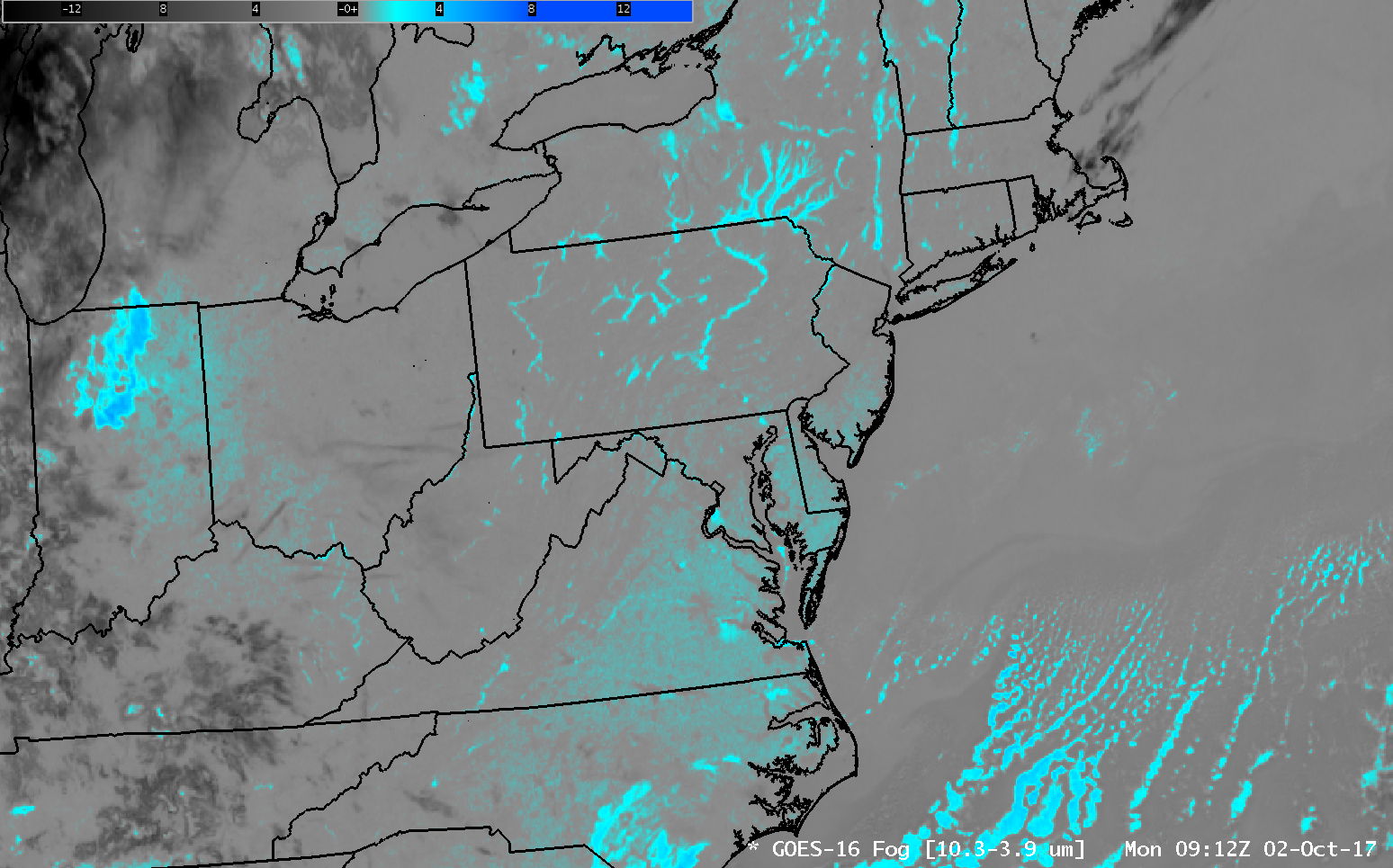
GOES-16 Brightness Temperature Difference (10.3 µm – 3.9 µm) at 0912 UTC on 2 October 2017 over the Mid-Atlantic States (click to enlarge)

GOES-16 data posted on this page are preliminary, non-operational and are undergoing testing.

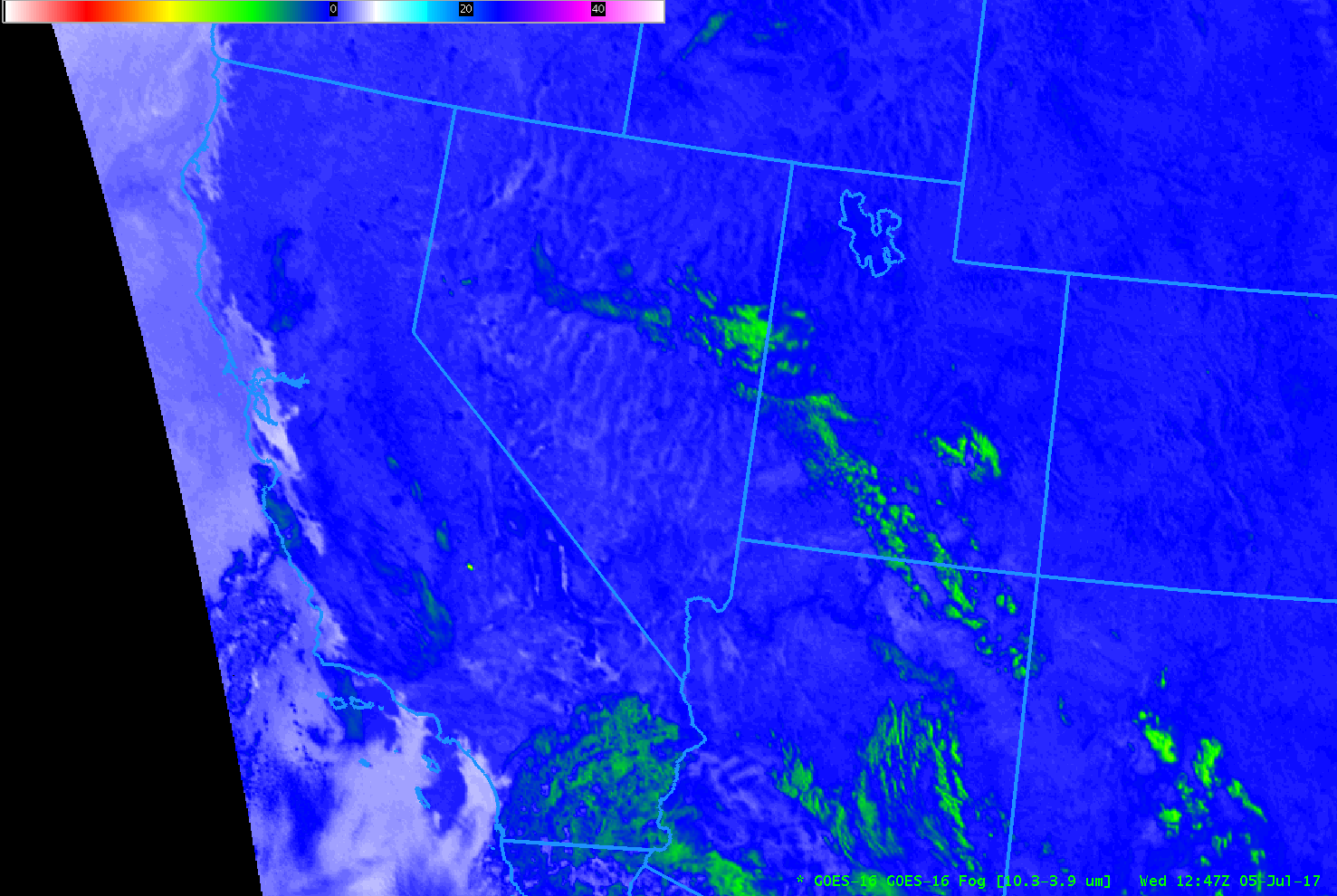
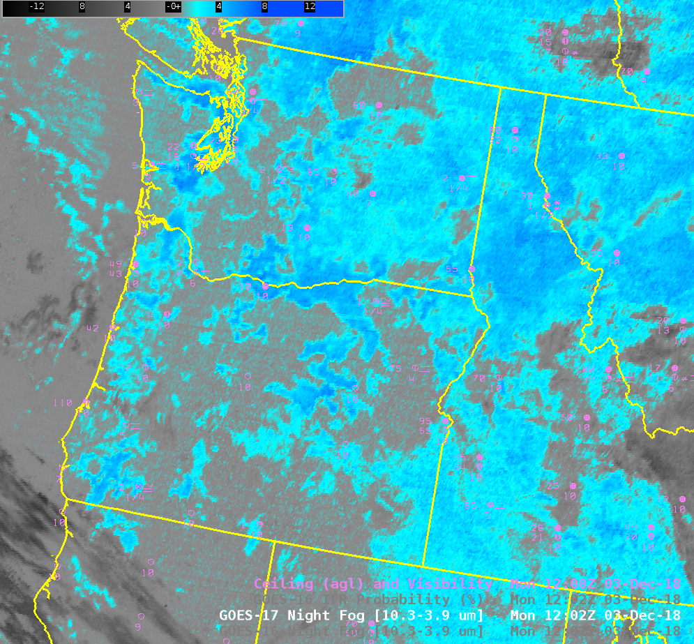
The images above show the GOES-16 Brightness Temperature Difference at the same time at two places over the United States: The mid-Atlantic States (above) and Oregon and surrounding States (below).  The ‘Fog’ Product, as this Brightness Temperature Difference is commonly called, in reality identifies only clouds that are made up of water droplets — that is, stratus.  A cloud made up of water droplets emits 10.3 µm radiation nearly as a blackbody does. Thus, the computation of Brightness Temperature — which computation assumes a blackbody emission — results is a temperature close to that which might be observed.  In contrast, those water droplets do not emit 3.9 µm radiation as a blackbody would.  Thus, the amount of radiation detected by the satellite is smaller than would be detected if blackbody emissions were occurring, and the computation of blackbody temperature therefore yields a colder temperature, and the brightness temperature difference field, above, will show clouds made up of water droplets as positive, or cyan in the enhancement above.

The River Valleys of the northeast show a very strong signal that suggests Radiation Fog is developing over the relatively warm waters in the Valleys.  The Delaware, Hudson, Mohawk, Connecticut, Susquehanna, Allegheny, Monongahela, and others — all show a signature that one would associate with fog.  A signal is also apparent from southern New Jersey southwestward through the Piedmont of North Carolina.  Would you expect there to be fog there as well, given the signal?

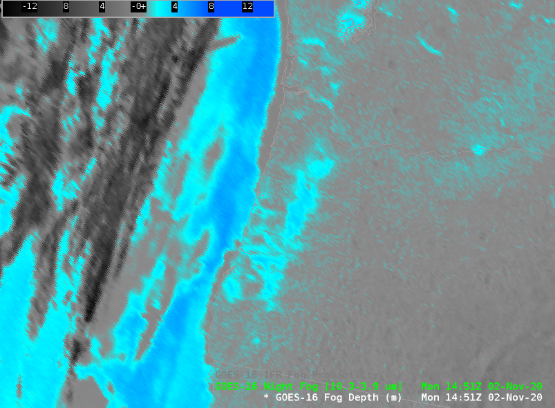
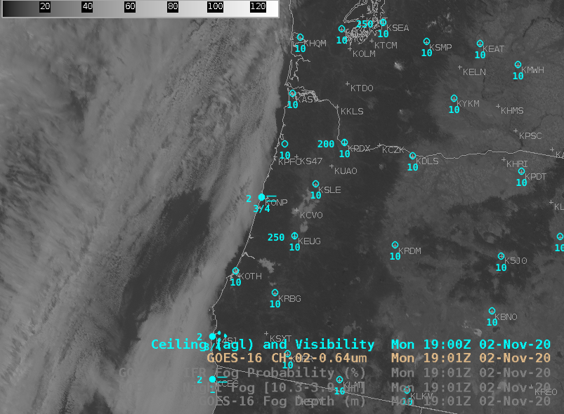
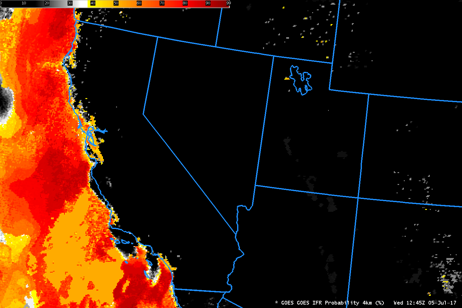
The State of Oregon at the same time shows a very strong signal in the ‘Fog’ Product.  A clue that this might be only stratus, and not visibility-restricting fog, lies in the structure of the clouds — they do not seem to be constrained by topographic features as is common with fog.

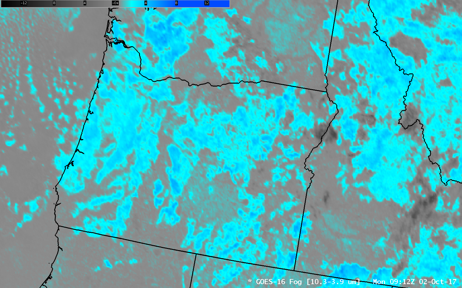
GOES-16 Brightness Temperature Difference (10.3 µm – 3.9 µm) at 0912 UTC on 2 October 2017 over Oregon and adjacent States (click to enlarge)

GOES-R IFR Probabilities are computed using Legacy GOES (GOES-13 and GOES-15) and Rapid Refresh model information; Preliminary IFR Probability fields computed with GOES-16 data are available here.  These GOES-16 fields should be available via LDM Request when GOES-16 becomes operational as GOES-East.

GOES-R IFR Probability Fields use both the Brightness Temperature Difference field (10.7 µm – 3.9 µm) from heritage GOES instruments and information about low-level saturation from Rapid Refresh Model output.  The horizontal resolution on GOES-13 and GOES-15 is coarser than on GOES-16 (4 kilometers at the sub-satellite point vs. 2 kilometers), so small river valleys will not be resolved.  (It is also difficult for the Rapid Refresh model to resolve small valleys).

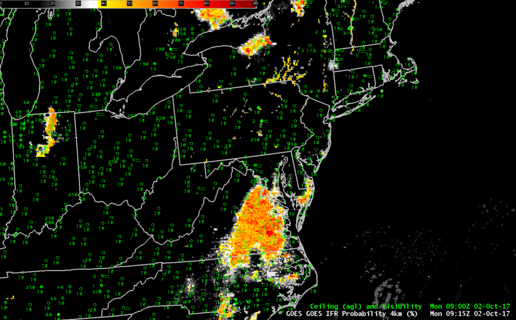
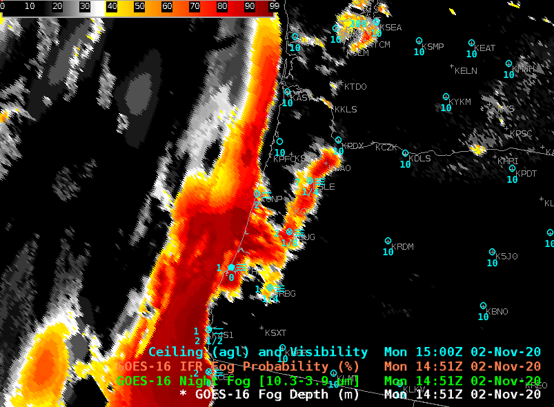
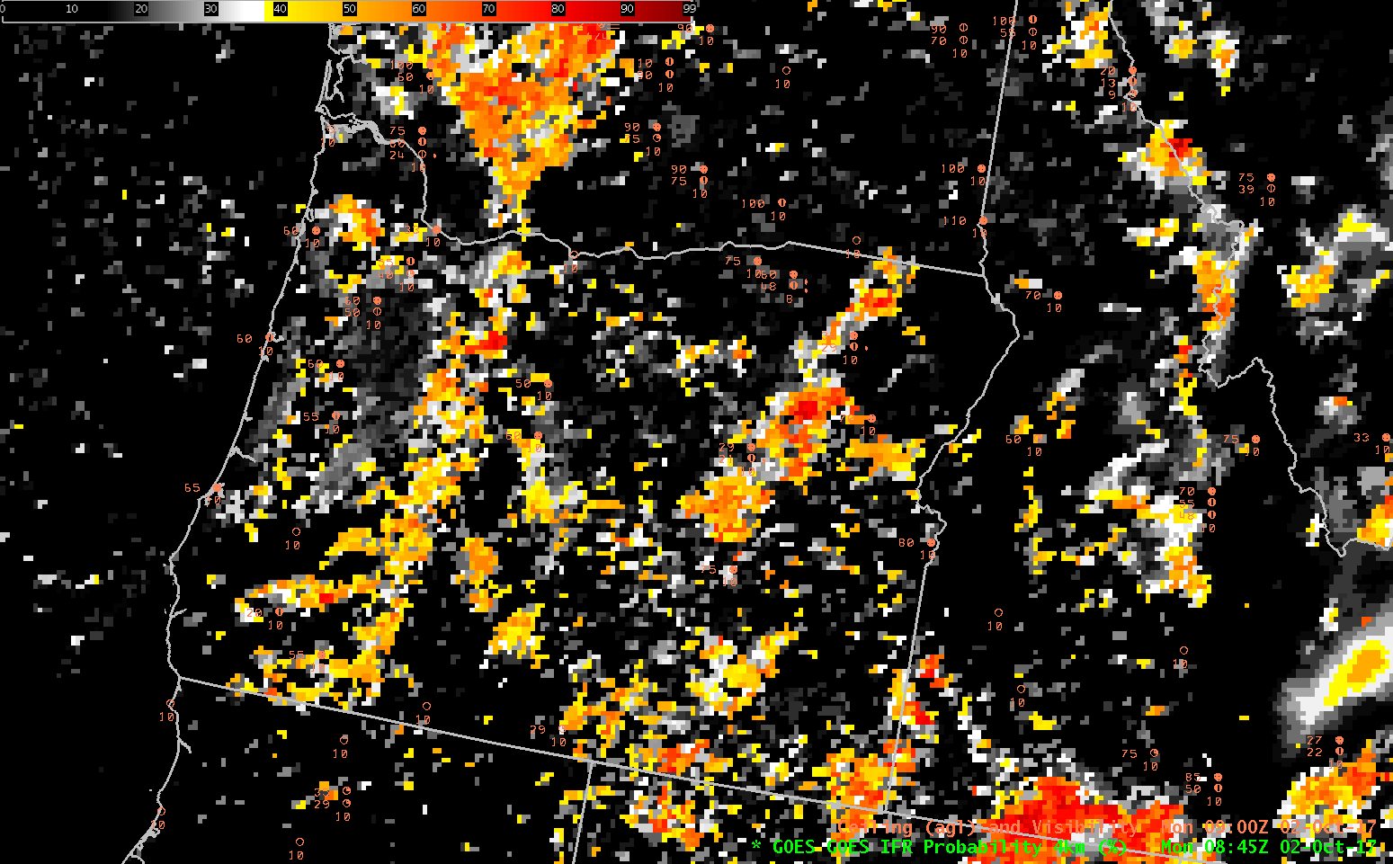
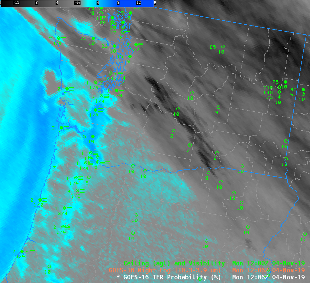
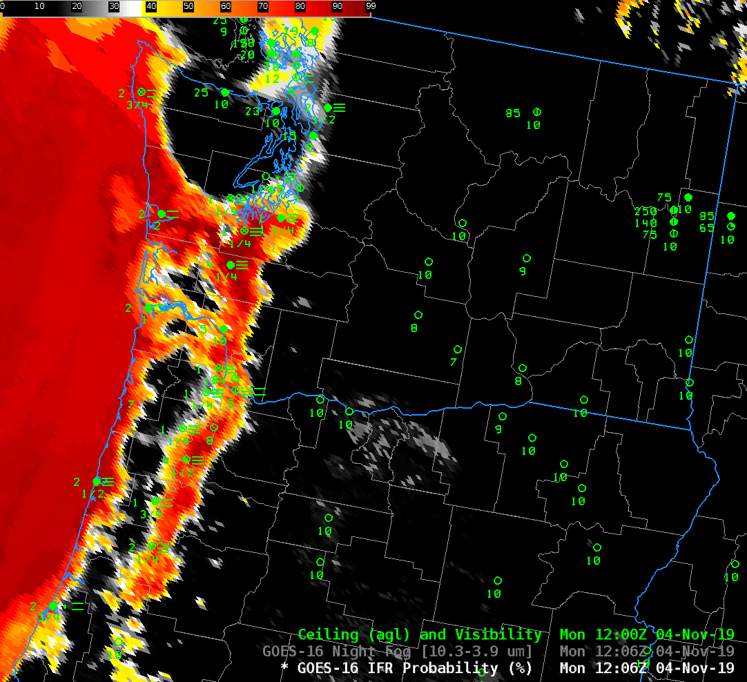
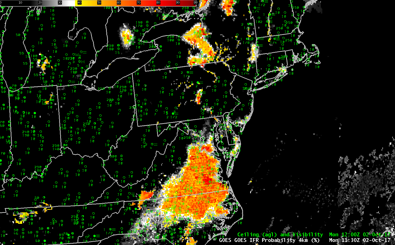
GOES-R IFR Probability fields at 0915 UTC, along with 0900 UTC surface observations of ceilings and visibility (Click to enlarge)

The IFR Probability Fields, above, show some signal over the river valleys of the northeast; that signal is mostly satellite-based, but the poor resolution of GOES-13 means that fog/stratus in the river valleys is not well-resolved. Still, a seasoned forecaster could likely interpret the small signals that are developing to mean fog is in the Valleys.  (And restrictions to ceilings and visibilities are certainly reported in the river valleys of the Mid-Atlantic and Northeast)   IFR Probabilities are also noticeable over southeast Virginia, although widespread surface observations showing IFR Conditions are not present.  (Such observations are somewhat more common near sunrise, at 1130 UTC).

IFR Probabilities are much less widespread over Oregon, with most of the signal over western Oregon related to the topography.  In this example, IFR Probabilities are ably screening out regions where elevated stratus is creating a strong signal for the satellite in the Brightness Temperature Difference field.

What GOES-16 Resolution will bring to IFR Probability

GOES-16 Brightness Temperature Difference field (10.3 µm – 3.9 µm) at 1247 UTC on 5 July 2017 (Click to enlarge)

GOES-16 data posted on this page are preliminary, non-operational data and are undergoing testing

GOES-R IFR Probabilities are computed using Legacy GOES (GOES-13 and GOES-15) and Rapid Refresh model information; GOES-16 data will be incorporated into the IFR Probability algorithm in late 2017

GOES-R IFR Probability fields continue to be created using legacy GOES (GOES-13 and GOES-15) data. This is slated to continue through late 2017. The toggle above, over Oregon, hints at how the change in resolution in GOES-16, even far from the sub-satellite point, will likely improve GOES-R IFR Probability performance in regions where topography can constrain low clouds and fog.  The GOES-16 Brightness Temperature Difference field, above, is color enhanced so that positive values (that is, where the brightness temperature at 10.3 µm is warmer than the 3.9 µm brightness temperature, which regions indicate cloud tops composed of water droplets, i.e., stratus) are whitish — and the data shows stratus/fog along the Oregon Coast, with fingers of fog advancing up small valleys.  The image below shows the GOES-R IFR Probability field for the same time (Click here for a toggle).

GOES-R IFR Probability fields show strong probabilities where the Brightness Temperature Difference field above is indicating low clouds.  This is not surprising as the morning fog on this date was not overlain by higher clouds.  However, the resolution inherent in the legacy GOES (inferior resolution compared to GOES-16), shows up plainly as a blocky field.  When GOES-R IFR Probability fields are computed using GOES-16 data, the IFR Probability field resolution will match the GOES-16 resolution.  (Click here for a aviationweather.gov observation of IFR / Low IFR conditions on the morning of 5 July).

GOES-R IFR Probability field computed from GOES-15 data at 1245 UTC on 5 July 2017 (Click to enlarge)

A similar set of figures for California at the same time is below.  The toggle is here, and the aviationweather.gov screen capture is here.

GOES-16 Brightness Temperature Difference field (10.3 µm – 3.9 µm) at 1247 UTC on 5 July 2017 (Click to enlarge)

GOES-R IFR Probability field computed from GOES-15 data at 1245 UTC on 5 July 2017 (Click to enlarge)