Category Archives: Appalachia

Resolution and Fog Detection in the mountains of the Appalachia

GOES-16 data posted on this page are preliminary, non-operational and are undergoing testing.

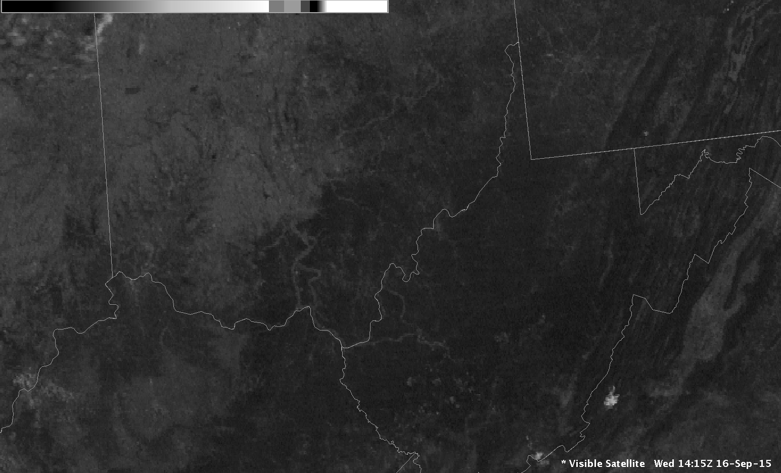
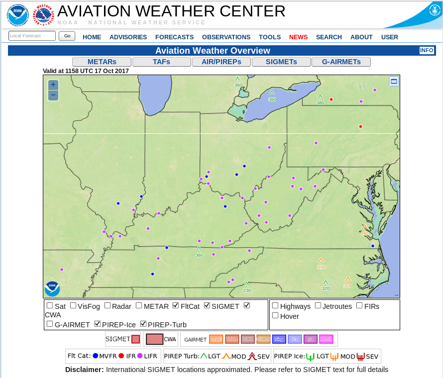
Clear skies and light winds allowed for the development of Radiation Fog over parts of West Virginia and surrounding states early on Tuesday 17 October 2017, and IFR conditions were widespread (Source).

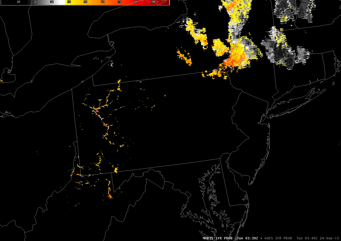
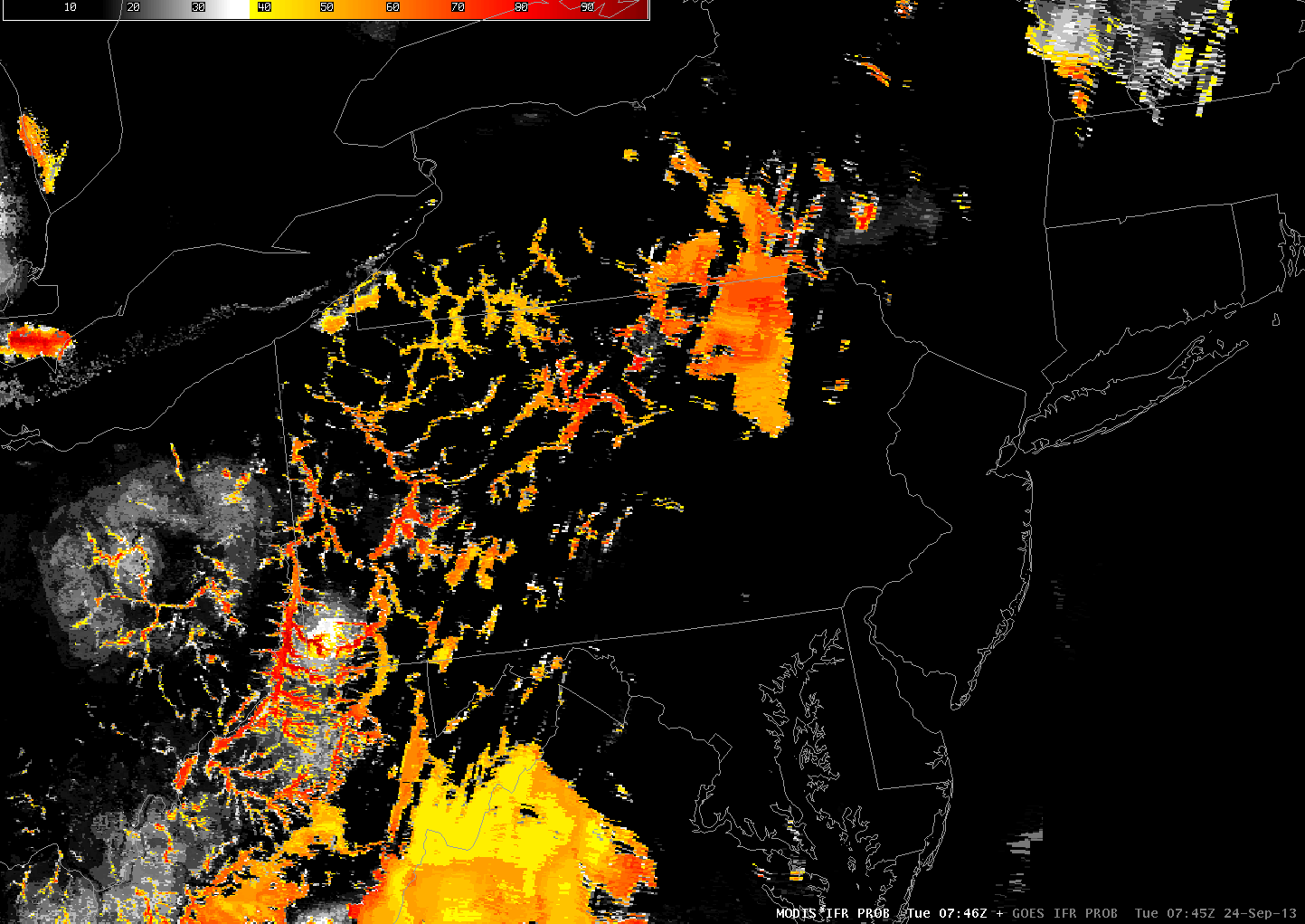
GOES-16 and GOES-13 both monitored this event, and toggles between the two brightness temperature difference fields, from 0315, 0415 and 0615 on 17 October, are shown below.  The better spatial resolution (and better precision) of the GOES-16 ABI is apparent in the imagery:  At 0415 UTC, GOES-16 is detecting river fog in many valleys in West Virginia and Kentucky, and is better resolving the detected fog over the Allegheny River in northwest Pennsylvania.  By 0615 UTC, the fog is also detected by GOES-13 — meaning it has increased in size so that the GOES-13 pixel size can detect it.  GOES-16 had a lead time of about 1-2 hours on GOES-13 in this case!

GOES-13 and GOES-16 Brightness Temperature Difference Fields, 0315 UTC on 17 October (Click to enlarge)

GOES-13 and GOES-16 Brightness Temperature Difference Fields, 0415 UTC on 17 October (Click to enlarge)

GOES-13 and GOES-16 Brightness Temperature Difference Fields, 0615 UTC on 17 October (Click to enlarge)

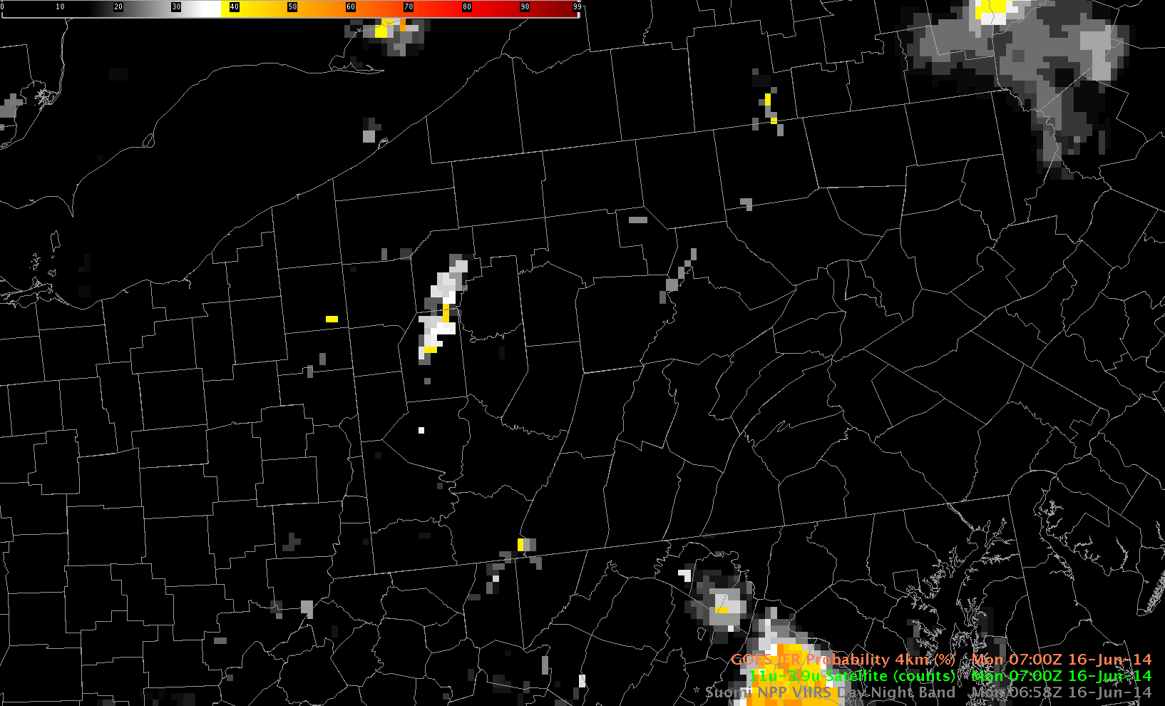
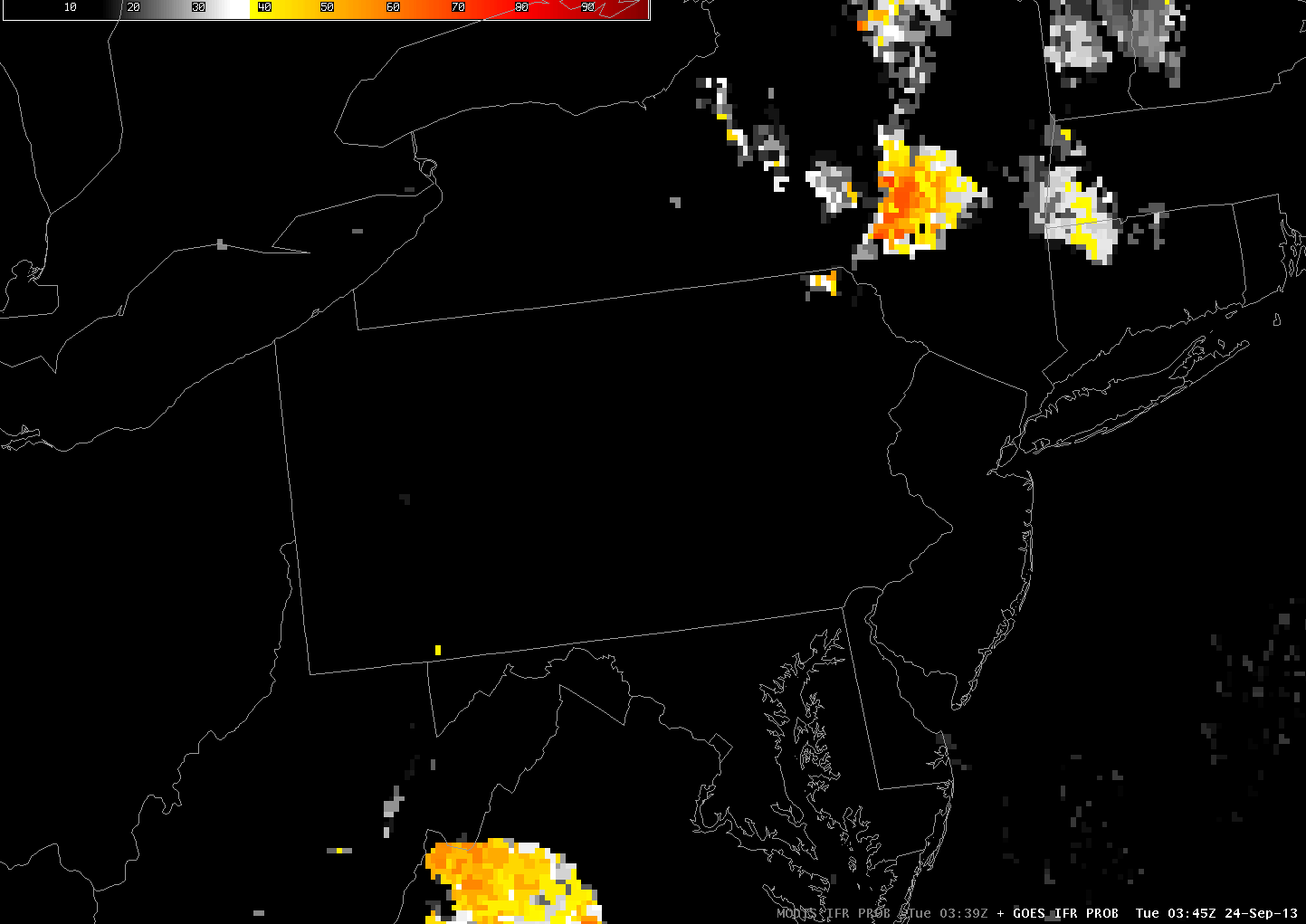
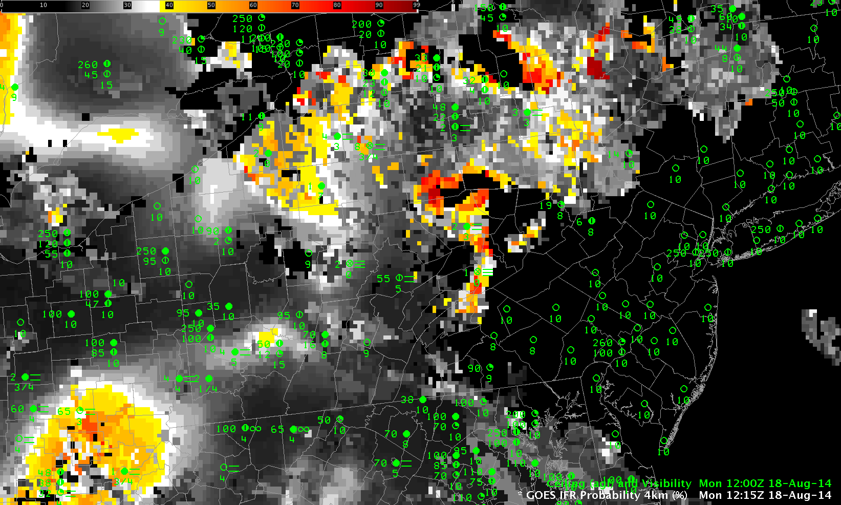
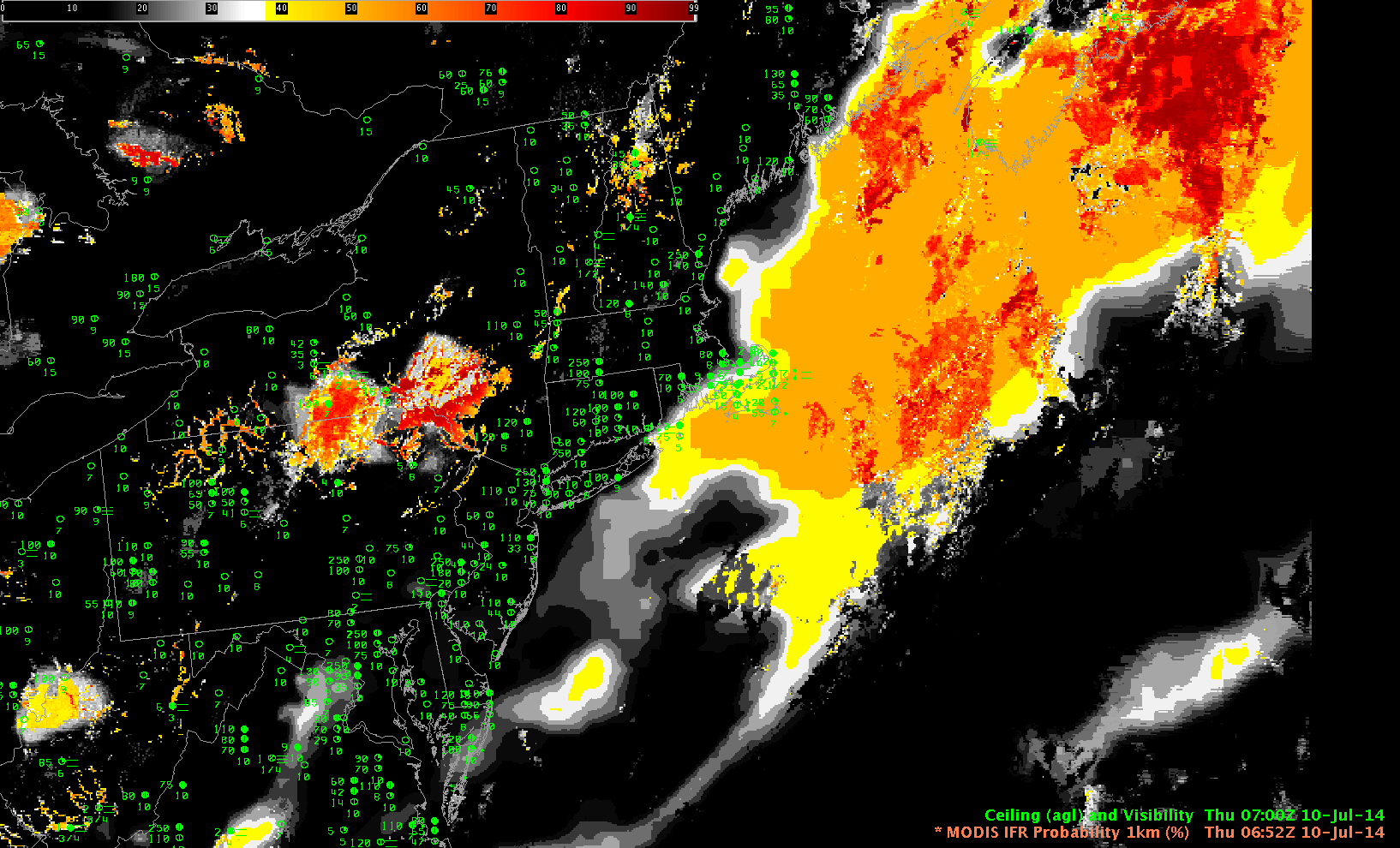
At present, GOES-R IFR Probabilities are created using GOES-13 data (or GOES-15 data for the western United States).  As might be expected, the GOES-R IFR Probabilities also lagged the GOES-16 Brightness Temperature Difference field in alerting to fog.  The short animation below shows values hourly from 0315-0615.  Very small IFR Probabilities are present at 0315 and 0415 — because, in part, the GOES-13 Imager cannot resolve the developing Fog/Stratus (and the Rapid Refresh model lacks the horizontal resolution to reproduce what is happening in narrow river valleys).  By 0515, and 0615 especially, GOES-R IFR probabilities are suggesting that a region of fog is likely.

One other thing to note:  There is a small signal in the brightness temperature difference field at 0315 UTC, above, in northwest Ohio in both GOES-13 and GOES-16 imagery.  There is no corresponding signal in the IFR Probability field.  The conclusion is that this is mid-level stratus that is not affecting surface visibility or ceilings.

GOES-R IFR Probabilities, hourly from 0315-0615 UTC on 17 October 2017 (Click to enlarge)

GOES-R IFR Probabilities, supplied via an LDM feed to National Weather Service Offices, will use GOES-13 (or GOES-15) imagery until GOES-16 is operational at 75.2 degrees West Longitude.  When GOES-16 is operational, GOES-R IFR Probabilities will use GOES-16 data, and that data will flow through the LDM.  In the meantime, GOES-16 IFR Probabilities can be viewed at this site.

Fog returned the following morning.  Link.

Resolution: GOES-R IFR Probability Fields and GOES-16 Data

GOES-R IFR Probabilities computed with GOES-13 and Rapid Refresh Data, Hourly from 0215-1115 UTC on 31 July 2017 (Click to enlarge)

GOES-R IFR Probabilities are computed using Legacy GOES (GOES-13 and GOES-15) and Rapid Refresh model information; GOES-16 data will be incorporated into the IFR Probability algorithm in late 2017

The animation above shows the evolution of GOES-R IFR Probability fields over West Virginia early on 31 July 2017, when IFR and Low IFR Conditions developed over much of the state. In addition to elevated probabilities over West Virginia, probabilities increased over eastern Virginia as well, where IFR conditions were not reported. The IFR probabilities over eastern Virginia diminished rapidly at sunrise, as indicated at the end of the animation.

Much of the fog on 31 July 2017 over West Virginia was valley fog. Legacy GOES (GOES-13 and GOES-15) has nominal 4-km resolution at the sub-satellite point, and this resolution can be insufficient to resolve the narrow valleys of the Appalachian Mountains.

GOES-16 data posted on this page are preliminary, non-operational and are undergoing testing

The GOES-16 Animation below shows the 10.3 µm – 3.9 µm Brightness Temperature Difference field for approximately the same time as above. The superior spatial resolution of GOES-16 is evident: tendrils of low clouds/fog are apparent in the animation that until sunrise highlights in green the clouds composed of water droplets (such as fog and stratus). A similar animation of the Nighttime Microphysics RGB Composite (here) similarly highlights stratus (as a whitish color) in the narrow river valleys.

GOES-16 Brightness Temperature Difference Fields (10.3 µm – 3.9 µm), hourly from 0312 – 1112 UTC on 31 July 2017 (Click to enlarge)

This Toggle between the GOES-R IFR Probability and the GOES-16 Brightness Temperature Difference field at 1015 UTC suggests how the IFR Probability Fields will better handle small valley fogs when GOES-16 data are used in the algorithm.

Cloud Thickness and Dissipation Time

Slide136

Dissipation time as a function of GOES-R Cloud Thickness

The chart above shows the relationship between the last pre-sunrise GOES-R Cloud Thickness product and Fog Dissipation time.  Observations of the last pre-sunrise GOES-R Cloud Thickness (developed from an empirical relationship between 3.9 µm emissivity and sodar-observed cloud thickness of the west coast of the USA) can be related to the dissipation time relative to the last observation of Cloud Thickness.  The scatterplot was developed using data mostly over the southeastern part of the USA, but also over the Great Plains.  However, it does have value in other geographic regions too, as shown below.

GOESR_CLDTHICK_IFRPROB_1100UTC_16sep2015toggle

GOES-R IFR Probabilities and GOES-R Cloud Thickness, 1100 UTC 16 September 2015 (Click to enlarge)

On 16 September, river fog developed over the Ohio River and its tributaries in Ohio, West Virginia and Pennsylvania. The toggle above shows GOES-R IFR Probability and GOES-R Cloud Thickness fields at 1100 UTC on 16 September.  This was the last pre-sunrise GOES-R Cloud Thickness over West Virginia (Indeed, the leading edge of twilight — where GOES-R Cloud Thickness is not computed — is apparent at the extreme eastern edge of the image, from Virginia up into central Pennsylvania). The GOES-R Cloud Thickness fields show largest values — around 800 feet — in/around the Ohio River between West Virginia and Ohio. The chart above suggest rapid dissipation. The best fit line (blue) suggests dissipation in about an hour, although there is considerable spread to the values, from 30 minutes up to almost 2-1/2 hours.

Almost two hours later (1245 UTC), fog is still present in isolated patches near the river, and GOES-R IFR Probability fields are suggesting fog is still present as well.  The horizontal extent of the GOES-R IFR Probability field is greatly reduced because visible imagery can be used after sunrise to screen out clear regions (Cloud-clearing in the algorithm is more effective).  By 1415 UTC (bottom), three hours after the GOES-R Cloud Thickness imagery above, all fog has evaporated.

GOES_VIS_GOESRIFRPROB_1245UTC_16sep2015toggle

GOES-R IFR Probabilities and GOES-13 Visible Imagery (with a low-light enhancement), 1245 UTC 16 September 2015 (Click to enlarge)

GOES_VIS_1415UTC_16sep2015

GOES-13 Visible Imagery, 1415 UTC 16 September 2015 (Click to enlarge)

MODIS resolution versus GOES resolution

WV_MODIS_GOES_IFRPROB_0315_11Sep2015toggle

MODIS-based (0300 UTC) and GOES-based (0315) UTC GOES-R IFR Probability fields on 11 September 2015 (Click to enlarge)

MODIS data (from Terra and Aqua) and GOES data can both be used to create GOES-R IFR Probability fields. The differences between the two data sources — especially spatial resolution — are obvious in the toggle above. MODIS data can capture the development of fingers of fog that develop in small river valleys, and GOES data cannot (although, of course, a forecaster with knowledge of the topography might appropriately tailor a forecast). In the toggle above, MODIS data capture the small tributaries of the Ohio River in Ohio and West Virginia that likely contain fog at 0300 UTC (11 PM local time). GOES data smear out that information. This is true later at night as well, below, at 0715 UTC. River valleys show higher IFR Probabilities than adjacent mountains. Valley fog is easier to delineate with MODIS data than with GOES data.

WV_MODIS_GOES_IFRPROB_0715_11Sep2015toggle

MODIS-based (0715 UTC) and GOES-based (0715) UTC GOES-R IFR Probability fields on 11 September 2015 (Click to enlarge)

Fog over Pennsylvania

GOES_IFR_PA_18August2014loop

GOES-R IFR Probabilities computed from GOES-13 data, hourly from 0500 through 1300 UTC 18 August 2014

River valley fog developed over Pennsylvania during the early morning hours of 18 August 2014, and the case is a good test of the GOES-R IFR Probability fields. IFR Probabilities are low at 0500 UTC (1 AM local time) and subsequently increase rapidly. In this case, the fields may be overpredicting where fog is present, as visible imagery just after sunrise suggest it was confined mostly to river valleys. In the animation above, the areal extent of the IFR Probabilities drops between 1100 UTC and 1215 UTC as the sun rises (the terminator is apparent in the 1100 UTC image, running from western Maryland north-northwestward to extreme western New York) and visible imagery can be used to more effectively cloud-clear the fields. A toggle between these two times is below. In this case, it is important to understand the geography underneath the IFR Probability field to hone the forecast.

GOES_IFR_PA_18August2014_1100-1215

GOES-R IFR Probabilities computed from GOES-13 data, at 1100 and 1215 UTC 18 August 2014

GOES13_BTD_18August2014loop

GOES-East Brightness Temperature Difference Fields (10.7µm – 3.9µm), hourly, from 0500-1100 UTC 18 August 2014

The Brightness Temperature Difference field, above, is the heritage method of detecting low stratus and inferring the presence of fog. Interpretation is complicated because high clouds (initially present over the southwestern portion of the scene, and moving eastward) prevent the satellite from viewing low clouds. In addition, as the sun rises (at the end of the animation, at 1100 UTC), solar radiation changes the character of the the brightness temperature difference field.

Data from the MODIS on board both Terra and Aqua can also be used to create both brightness temperature difference fields and IFR Probability fields. The toggle below, using ~0700 UTC data from GOES and from MODIS, shows the distinct advantage present in the MODIS field’s superior spatial resolution (1-km at sub-satellite point vs. 4-km at the sub-satellite point for GOES). River valleys are more evident in the MODIS data, by far, than in the GOES data.

GOES_MODIS_IFR_18August2014_07

GOES-R IFR Probabilities computed from GOES-13 data and from MODIS data, at 0700 UTC 18 August 2014

The Day-Night band on Suomi NPP at 0718 UTC showed that the densest fog was largely confined to river valleys.

SNPP_DNB_18August2014_0718UTC

Suomi NPP Day/Night Band, 0718 UTC on 18 August 2014

An animation of the fog burning off from GOES-14 (in special 1-minute SRSO-R scanning operations) is available here. It’s also on YouTube.

Distinguishing between stratus and fog over Pennsylvania

SNPP_11.35_0609_0747_10July2014

Suomi NPP 11.35 µm Infrared Imagery at 0609 and 0752 UTC, 10 July 2014 (Click to enlarge)

The orbital geometry of Suomi NPP allowed two high-resolution images of Pennsyvlania early in the morning of the 10th of July 2014. Can you tell from the imagery above if there is fog/stratus in the river valleys of Pennsyvlania? Are the relatively cool clouds from Pittsburgh northeastward towards Elmira, NY obstructing visibilities? Based on the IR (11.35 µm for Suomi NPP) imagery alone, above, that is a difficult question to answer. Historically, the brightness temperature difference between the longwave IR (11.35 µm) and the shortwave IR (3.74 µm) has been used to indentify water-based clouds. Imagery from Suomi NPP, below, highlights where water-based clouds (like stratus) exist. If the clouds are the same temperature as the surrounding land (likely the case for river fog), a single 11.35-µm image is of little help in identifying the clouds.

SNPP_11.35-3.74_0609-0747UTC_10July2014

Suomi NPP 11.35 – 3.74 µm Brightness Temperature Difference at 0609 and 0752 UTC, 10 July 2014 (Click to enlarge)

The Day-Night band can also highlight where clouds exist, because lunar illumination reflects well off clouds. A 3/4-full moon ably illuminates the scene at 0609 UTC, but that moon has set at 0747 UTC and the Clouds are harder to see.

SNPP_DNB_0609-0747UTC_10July2014

Suomi NPP Day/Night Band at 0609 and 0752 UTC, 10 July 2014 (Click to enlarge)

Both the Day/Night band and the Brightness Temperature Difference Fields (and any Infrared image) gives information about the top of the cloud. Fog existence is difficult to discern only from satellite data because the bottom of the cloud is not sampled. This is why a fused product (such as IFR Probability) that includes surface information (in the case of IFR Probability from the Rapid Refresh Model) is desirable. MODIS data can be used to compute IFR Probability, and a MODIS-carrying Aqua pass occurred in between the two Suomi NPP Passes shown above.

MODIS_BTD_IFR_0652UTC_10July2014

MODIS 11 – 3.9 µm Brightness Temperature Difference and IFR Probability at 0652 UTC, 10 July 2014 (Click to enlarge)

In the two images above, note how the IFR Probability Fields de-emphasize the low cloud areas that stretch northeastward from Pittsburgh towards Elmira. This is likely mid-level stratus. River Fog over northeast Pennsylvania is highlighted in the IFR Probability fields (and in the brightness temperature difference field). This image, which shows the GOES-based IFR Probability field at 0645 UTC, highlights the power of MODIS’ superior spatial resolution in the early detection of small-scale fog. The large region of reduced visibility around Elmira NY (meager surface observations suggest this large region of fog verified) appears in both MODIS- and GOES-based IFR Probability fields. Only the MODIS-based IFR Probability field, however, has a distinct river-valley signal over northeast Pennsylvania.

MODIS and GOES IFR Probability both suggest IFR conditions may be occurring over the Atlantic Ocean. The brightness temperature difference field shows no low cloud signal there because of a cirrus shield. IFR Probability gives a signal of fog here based on information from the Rapid Refresh.

Fog in the Valleys of Pennsylvania and New York

PA_SNPP_DNB_BTD_0658UTC_16June2014

Suomi/NPP Day/Night Band and Brightness Temperature Difference (11.35 – 3.74) at 0658 UTC on 16 June 2014 (Click to enlarge)

Suomi/NPP Day/Night band “Visible Imagery at Night” from last night at 3 AM EDT over Pennsylvania and surrounding states shows cloud formation in the river valleys of Pennsylvania and New York. The brightness temperature difference also shows these cloud formations, but note over eastern New York how high cirrus prevents the detection of low clouds in river valleys using the brightness temperature difference field, but the cirrus is thin enough that the Day/Night band does show the low clouds. The brightness temperature difference field can show where clouds are present in regions where city lights in the day/night band might appear similar to clouds on a night when lunar illumination is strong (as was the case on 16 June 2014) — for example, along US Highway 220 from Lock Haven to Jersey Shore and Williamsport in southern Clinton and Lycoming Counties.

Of course, the Suomi/NPP satellite is seeing the top of the cloud, so it can be difficult to infer ceiling and visibility obstructions from these data. The GOES-based IFR Probability field from about the same time, below, shows hints of visibility restrictions, but the coarser resolution of GOES-13 (compared to Suomi/NPP) limits the ability of GOES to herald the development of fog. In addition, the 13-km resolution of the Rapid Refresh model data that are also used in the GOES-R IFR Probability fields is insufficient to resolve the small river valleys (such as Pine Creek that shows up very well in the S/NPP imagery in western Lycoming County). Portions of the Susquehanna River basins do show marginally enhanced probabilities, certainly something that would alert a forecaster to the possibilities of fog.

PA_IFRProbGOES_0700UTC_16June2014

GOES-based IFR Probabilities, 0700 UTC on 16 June 2014 (Click to enlarge)

MODIS data can also be used to produce IFR Probabilities at infrequent intervals, but a timely overpass at 0744 UTC shows high probabilities in most of the river valleys of central Pennsylvania and upstate New York, with the highest probabilities near Elmira, NY.

MODIS_IFR_0744UTC_16June2014

MODIS-based IFR Probabilities, 0744 UTC on 16 June 2014 (Click to enlarge)

The GOES-R IFR Probabilities at 1000 UTC, below, show evidence that the fog/low stratus have become widespread enough in river valleys to be detected even by GOES. Elmira, NY, is reporting IFR conditions, and such conditions are also likely elsewhere in the valleys (although no observations are available to confirm that).

PA_IFRPROB_1000UTC_16June2014

GOES-based IFR Probabilities, 1000 UTC on 16 June 2014 (Click to enlarge)

Use timely polar-orbiting satellite data — with high resolution — to confirm suspicions of developing fog in river valleys. Then monitor the situation with the good temporal resolution of GOES. During the GOES-R era, geostationary satellite spatial resolution will be increased and fog detection from GOES-R should occur with better lead time.

Benefits of Resolution with a Polar-orbiting satellite

US_11-3_GOES_IFR_201401516_0630toggle

Toggle between GOES-13 Brightness Temperature Difference (10.7µm – 3.9µm) and GOES-R IFR Probability over Kentucky and surrounding states. Surface observations of ceiling heights and visibility are included, 0630 UTC 16 May 2014 (Click to enlarge)

The toggle above highlights a strength of the GOES-R IFR Probability fields compared to the GOES Brightness Temperature Difference when it comes to detecting low fog/stratus. The Brightness Temperature Difference field only sees the top of the cloud. In the toggle above, the region of elevated stratus, the stratus over western Virginia and western West Virginia is highlighted, but those clouds are unimportant for aviation/transportation, and IFR Probability fields ignore that region (save for the spine of the Appalachians where the mountains are rising up into the clouds, so ceilings are near the surface).

There are heightened IFR Probabilities in/around KEKQ (Monticello, Kentucky) at 0630 UTC: what is the character of that fog? It’s difficult to tell with the coarse GOES resolution (although someone familiar with the topography of eastern Kentucky might guess).

The imagery below toggle between the high-resolution (1-km) Suomi/NPP VIIRS Brightness Temperature Difference (11µm – 3.74µm) and the Day/Night Band at 0638 UTC. The higher resolution imagery allows the dendritic nature of the valley fog to appear in a way that is impossible with the coarser-resolution GOES data. Fog is initially developing in river valleys. Both the Brightness Temperature Difference and Day/Night imagery, however, are seeing only the top of the cloud and are not giving information about the likelihood of fog. But the cloud structure would alert a forecaster to the probability of developing fog (as does the time trend in the GOES-R IFR Probability fields).

Note how the cirrus shield east of the Appalachians shows up distinctly in both GOES and VIIRS brightness temperature difference fields. High clouds such as those prevent the satellite detection of fog/stratus at low levels. In those cases, only the IFR Probability field has a chance to detect fog if it is present.

VIIRS_DNB_FOG_20140516_0638toggle

Suomi/NPP Brightness Temperature Difference (11.0µm – 3.74µm) and Day/Night Band from VIIRS, 0638 UTC 16 MAy 2014 (Click to enlarge)

By 1000 UTC, the fog that was initially confined to river valleys over central Kentucky has expanded. In this case, Suomi/NPP data (or the trending of the GOES data) gives a forecaster a heads up on the development of overnight fog.

GOES_IFR_PROB_20140516_1000

GOES-R IFR Probability over Kentucky and surrounding states. Surface observations of ceiling heights and visibility are included, 1000 UTC 16 May 2014 (Click to enlarge)

Dense fog on the East Coast

VIIRS_DNB_FOG_20140115toggle

GOES-East IFR Probabilities and surface plots of visibilities/ceilings at 0615 UTC 15 January (Upper Left), GOES-East Brightness Temperature Difference (10.7 µm – 3.9 µm), 0615 UTC 15 January (Upper Right), GOES-R Cloud Thickness, 0615 UTC 15 January (Lower Left), and Suomi/NPP Day/Night Band and Brightness Temperature Difference toggle (11.35 µm – 3.74 µm), 0605 UTC 15 January (Lower Right)(click image to enlarge)

The image above documents the GOES-R IFR Probability field during a fog event over the East Coast. Note how the IFR Probability field shows more horizontal uniformity than the traditional brightness temperature difference field over eastern Pennsylvania (where IFR conditions are reported). For example, both Selinsgrove along the Susquehanna and Reading in south-central Pennsylvania report IFR conditions in regions where the IFR Probability field has a strong return, but where the brightness temperature difference field’s diagnosis is less certain.

The Suomi/NPP field demonstrates the importance of higher resolution from polar orbiting satellites. Both the Day/Night Band and the brightness temperature difference fields suggest the presence of river valley fog over the West Branch of the Susquehanna and its many tributaries in central Pennsylvania. This continues at 0743 UTC, below, when Suomi/NPP’s subsequent overpass also viewed the Susquehanna valley. At both times, the river fog is too small-scale to be detected with GOES-13’s nominal 4-km pixel size.

VIIRS_DNB_FOG_20140115toggle

GOES-East IFR Probabilities and surface plots of visibilities/ceilings at 0745 UTC 15 January (Upper Left), GOES-East Brightness Temperature Difference (10.7 µm – 3.9 µm), 0745 UTC 15 January (Upper Right), GOES-R Cloud Thickness, 0745 UTC 15 January (Lower Left), and Suomi/NPP Day/Night Band and Brightness Temperature Difference toggle (11.35 µm – 3.74 µm), 0743 UTC 15 January (Lower Right)(click image to enlarge)

The animation of the fields, below, done to demonstrate the importance of GOES-13’s temporal resolution, shows how the GOES-R IFR Probability field accurately captures the extent of the fog, even as the sun rises and causes the sign of the brightness temperature difference to flip. The traditional brightness temperature difference field has difficulty both in maintaining a signal through sunrise, and it diagnosing the region of fog/low stratus over northcentral Pennsylvania in and around the Poconos and in the Susquehanna River valley. The IFR Probability field has a minimum over/around Mt. Pocono, where IFR conditions are not observed until close to sunrise. IFR probabilities are small over Altoona, where the brightness temperature difference field shows a strong signal developing late at night (and where observations suggest an elevated stratus deck). In this region, although the satellite suggests fog might be present, model conditions do not agree, and IFR Probabilities are correctly minimized.

GOES-R Cloud thickness suggests that the thickest blanket of fog is over New Jersey. This diagnosis continues up through the twilight conditions of sunrise, at which point Cloud thicknesses are no longer diagnosed.

GOES_IFR_PROB_20140115loop

GOES-East IFR Probabilities and surface plots of visibilities/ceilings (Upper Left), GOES-East Brightness Temperature Difference (10.7 µm – 3.9 µm) (Upper Right), GOES-R Cloud Thickness (Lower Left), and GOES-East Water Vapor (6.7 µm), all times as indicated (Lower Right)(click image to enlarge)

Resolution and Valleys

GOES_IFR_PROB_20130924_0345

GOES-based GOES-R IFR Probabilities, 0345 UTC 24 September 2013 (click image to enlarge)

Consider the GOES-R IFR Probabilities computed from GOES-East data (and Rapid Refresh data) above. How confident are you that, at 0345 UTC, fog is forming in river valleys of western Pennsylvania? Is the likelihood the same in the southern part of the state (say, along the Monongahela River) as in the northern part of the state (along the Clarion or Allegheny Rivers)? GOES resolution in the infrared channels is 4 km at the sub-satellite point. In Pennsylvania, resolution is degraded to 5 or so kilometers. The knowledge of pixel size should color your interpretation of the GOES-R IFR Probabilities (and of the brightness temperature difference field computed from GOES). The MODIS-based GOES-R IFR Probabilities from 0339 UTC, below, show a ribbon of high probabilities over many of the river valleys of Pennsylvania. This 1-km resolution information is handy at capturing the initial development of fog and low stratus.

MODIS_IFR_PROB_20130924_0339

MODIS-based GOES-R IFR Probabilities, 0339 UTC 24 September 2013 (click image to enlarge)

VIIRS_DNB__REF_20130924LakeErieLoop

Suomi/NPP VIIRS Day/Night band imagery, 0640 and 0820 UTC 24 September 2013 (click image to enlarge)

Day/Night band imagery over Pennsylvania and New York shows the expansion of fog coverage between successive Polar Passes, at 0640 and 0820 UTC. The imagery below shows the corresponding GOES-based GOES-R IFR Probabilities at those two times. The large cloud features over northeast Pennsylvania and the Southern Tier of New York are captured well by the GOES-based fields; the river valley fogs are not captured quite so well because of resolution limitations.

GOES_IFR_PROB_20130924loop

GOES-based GOES-R IFR Probabilities, 0645 and 0815 UTC 24 September 2013 (click image to enlarge)

A MODIS-based IFR probability field, below, far better represents the presence of River Valley fogs at 0746 UTC than the GOES-based IFR Probability Field, bottom, from 0745 UTC. (These times are between the two times in the GOES-R IFR Probability animation above) A good method for monitoring fog would incorporate the fine spatial resolution at the start of the fog event to ascertain which river valleys are starting first to become fog-bound. The good temporal resolution of GOES data is then used to outline the evolution of the event. Periodic Polar Orbiter passes from Terra, Aqua of Suomi/NPP as the fog event is occurring can confirm the GOES-based predictions of the evolution of fog.

MODIS_IFR_PROB_20130924_0746

MODIS-based GOES-R IFR Probabilities, 0746 UTC 24 September 2013 (click image to enlarge)

GOES_IFR_PROB_20130924_0745

GOES-based GOES-R IFR Probabilities, 0745 UTC 24 September 2013 (click image to enlarge)