Fog/Low Stratus in eastern Washington State

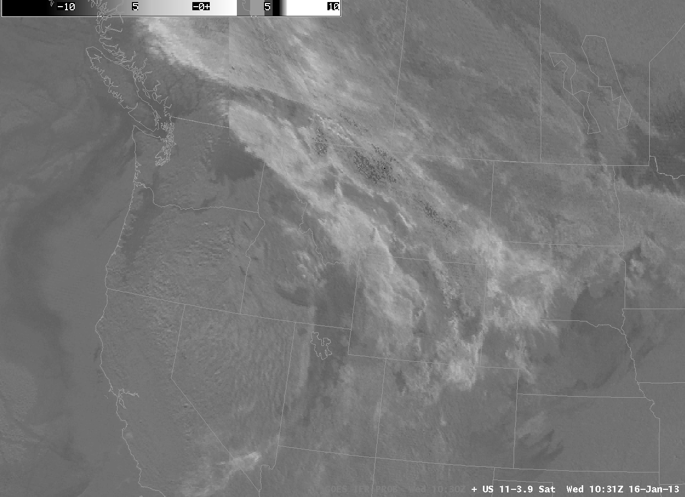
Brightness Temperature Difference plot over the NW USA, 1031 UTC 16 January

The plot above shows the default enhancement the brightness temperature difference product traditionally used to highlight regions of low clouds and fog.  The greyscale nature of the product can make interpretation difficult.  However, if a suitable enhancement is applied (below), such that fog and low clouds are enhanced, interpretation is easier.

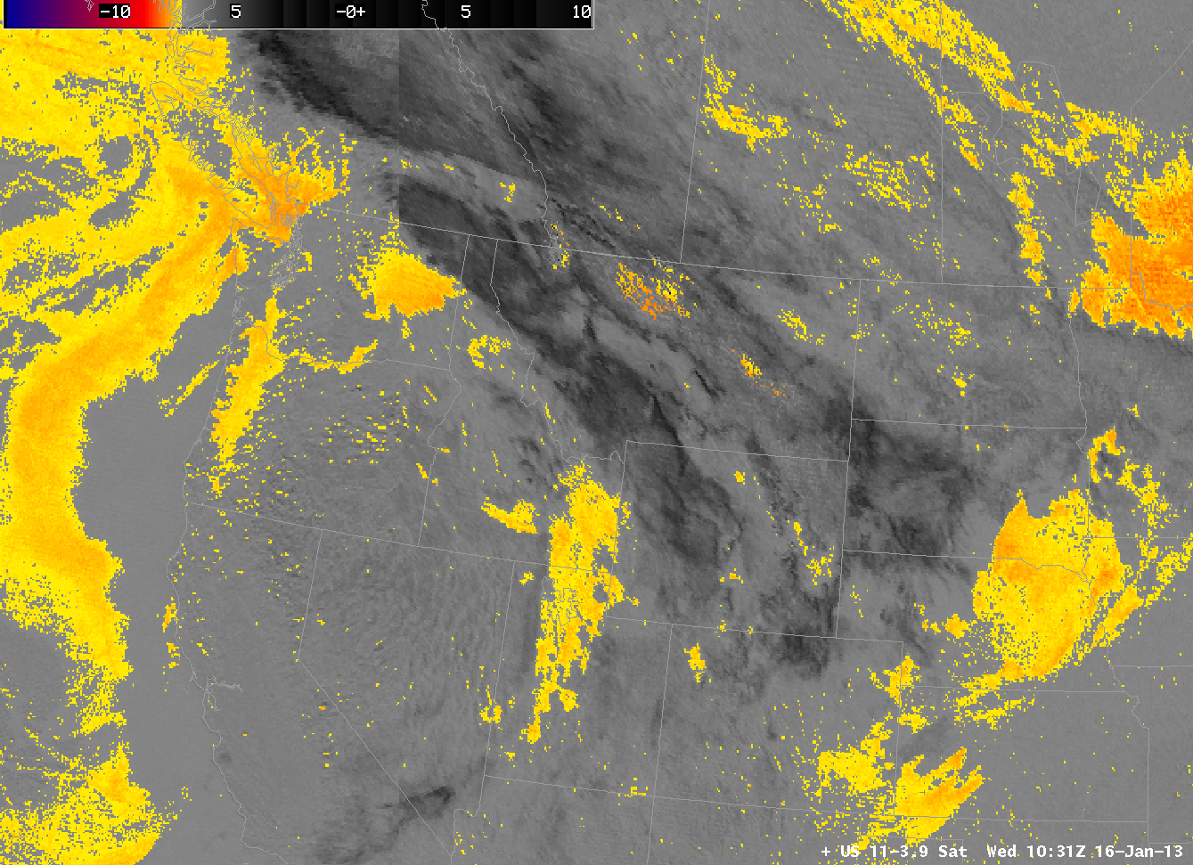
As above, but color-enhanced.

This image suggests the presence of fog or low stratus (or both) off the west coast of the US, in and around Salt Lake City, near Spokane, and in the Willamette Valley and Columbia River Valley.  It is difficult to tell if the regions are associated with restrictions in visibility because an elevated stratus deck and a fog bank look very similar in the brightness temperature difference field.  Therefore, the GOES-R Fog/Low Stratus IFR Probability field was developed to highlight regions where IFR conditions are most likely.  That product is shown below.

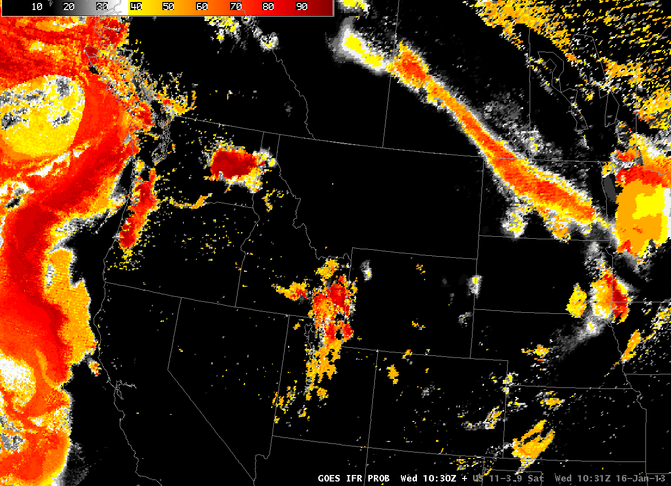
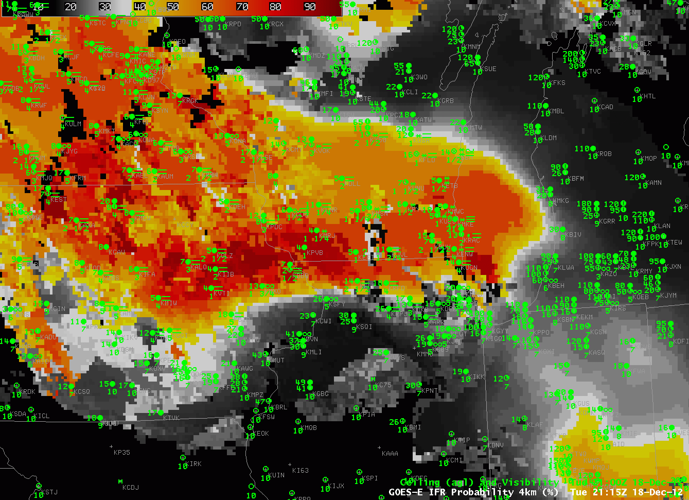
GOES-R IFR Probabilities, 1030 UTC on 16 January

Compare the IFR probability field to the Brightness Temperature Difference field above it.  Several things are apparent.  Highest probabilities for visibility restrictions are centered near Spokane, WA.  There is a region of higher IFR probabilities in North Dakota that is missing entirely in the Brightness Temperature Difference product.  IFR probabilities over Utah vary more than the Brightness Temperature Difference signal.  The differences all arise from the model data that are used to better highlight where low-level saturation is occurring.

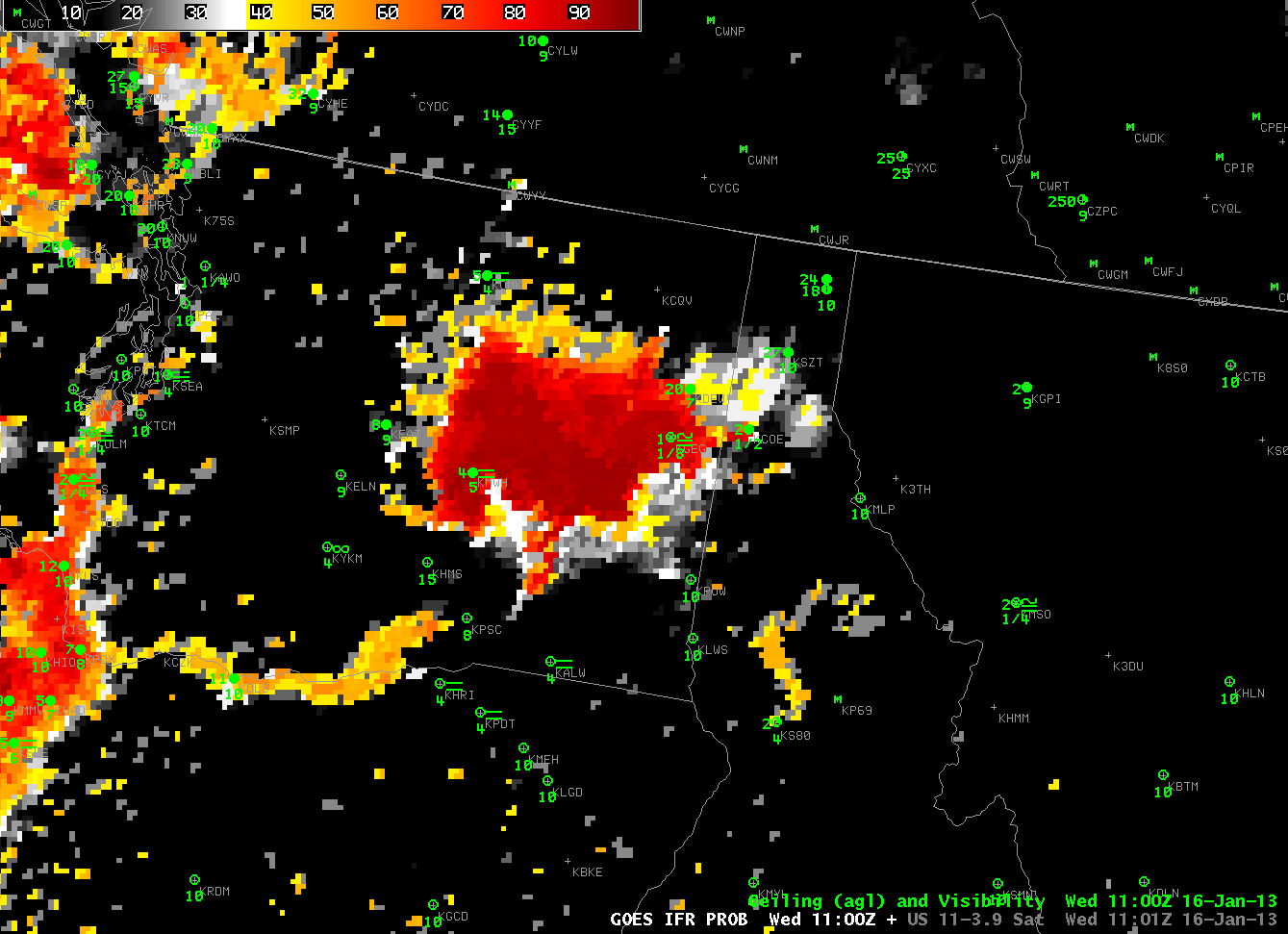
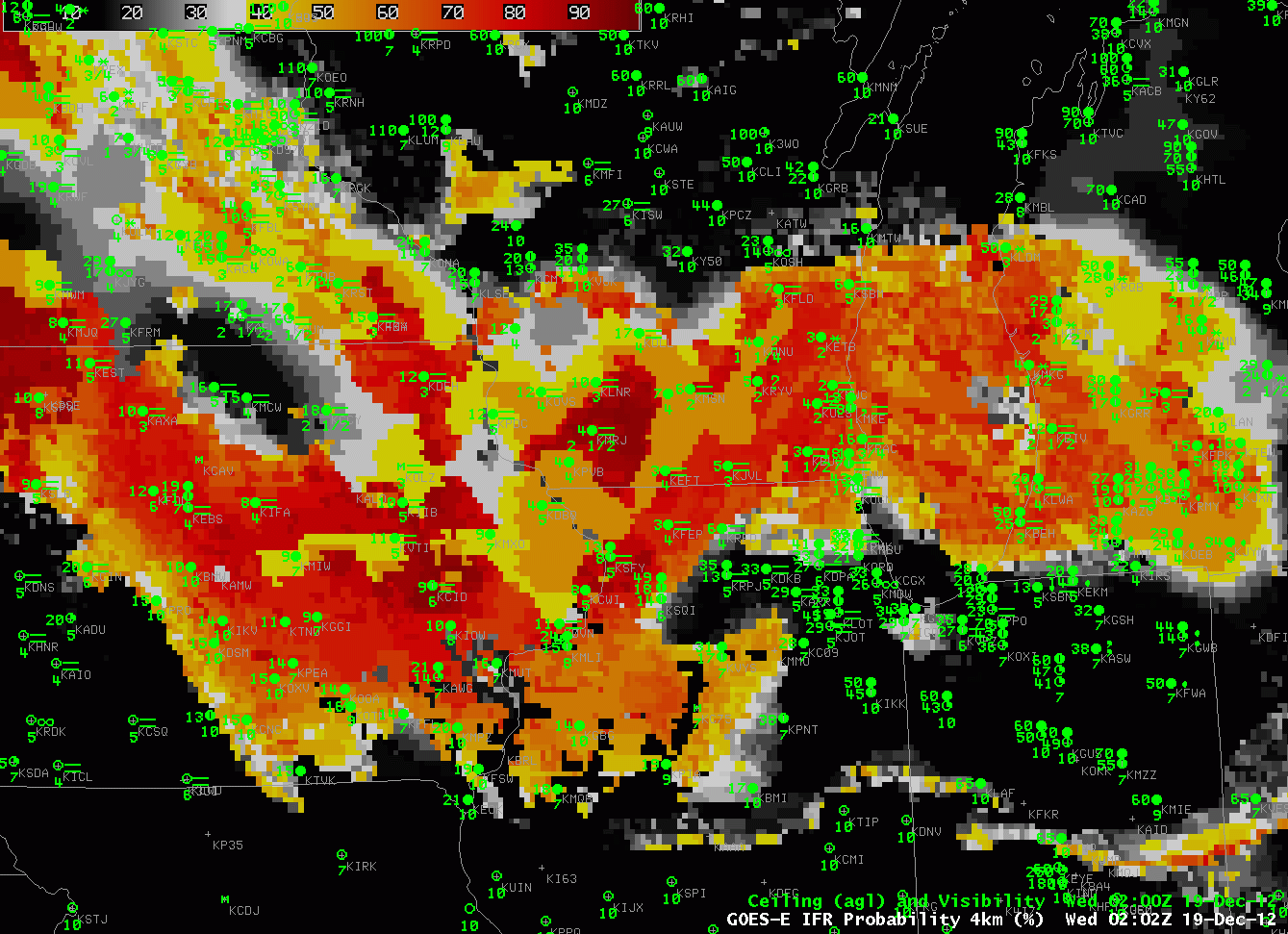
IFR Probabilities and observations of Ceilings/visibilities from 1100 UTC on 16 January.

This zoomed-in imagery shows that, indeed, visibility restrictions (IFR conditions) are occurring in eastern Washington.  The strength of the fused product is that is provide a coherent signal over a larger area, so you can better define the region of IFR conditions than is possible with surface observations alone.  The region of higher IFR probabilities over North Dakota is also associated with IFR and near-IFR conditions in a northwest-southeast oriented strip including Harvey and Jamestown, ND (not shown).

IFR conditions with multiple clouds layers over the southeast US

GOES-R IFR Probabilities from GOES-East (Upper Left), GOES-East Brightness Temperature Differences (Upper Right), GOES-R Cloud Thickness (Lower Left), Surface Observations of Ceilings and Visibility (Lower Right), all at 1000 UTC on 16 January 2013

A slowly-moving weather system brought extensive cloudiness and IFR and near-IFR conditions over the southeast part of the United States again on January 16, and provided a good example of how the fused nature of the GOES-R Fog/Low Stratus product — combining both satellite and model information — yields a better signal (than is available from the traditional brightness temperature difference product) of where fog and low stratus are most likely.  The imagery from 1000 UTC, which is characteristic of the entire event, shows a brightness temperature difference signal over the southest that is consistent with the observed multiple cloud layers.  Such a cloud configuration makes it very difficult to relate the brightness temperature difference signal to surface observations.  in contrast, the IFR Probability field show a widespread region of high probabilities, overlapping the regions of near-IFR and IFR observations over Tennessee, and points south.  Cloud thickness, which is computed only where single water-cloud layers are detected from satellite, indicates cloud thicknesses around 1000 feet.  Note that where the cloud thickness is diagnosed, in general, IFR probabilities are relatively larger.  This is because IFR probabilities combine satellite predictors and model predictors.  If the satellite predictors cannot be generated because of multiple cloud layers and/or a single high cirrus deck, then only the model predictors are driving the IFR probability value, and the probability will therefore be lower.  This is the case over western Tennessee and central Georgia.

Dense Fog Event Over the Upper Midwest U.S.

False color image of  a winter storm system moving across the upper Midwest U.S. on 11 January 2013.

A strong winter storm system moved over the upper Midwest on 11 January 2013 bringing heavy snow to the Dakotas. Rain and warm air moved in over the mostly snow covered areas of eastern Nebraska, Minnesota, Iowa, Wisconsin and northern Illinois resulting in a large area of locally dense fog. GOES-R IFR probabilities were used to monitor the large-scale event as it moved over the Upper Midwest U.S.

Due to a large amount of overlaying clouds a satellite only product such as the traditionally-used 11-3.9 micron Brightness Temperature Difference (BTD) only sees the top cloud layer and therefore can not detect fog/low stratus (FLS) beneath. The GOES-R IFR probabilities, however, combine both satellite and mesoscale NWP model data to create a blended product that can estimate the probability that IFR conditions are present even where overlaying clouds obscure all or part of the scene. This animation of the weather system shows that the traditional 11-3.9 micron BTD product only detects a small portion of the fog event, confirmed by the surface observations of ceiling and visibility. The GOES-R FLS product provides relatively high probabilities (>50%) that IFR conditions are present over the entire extent of the fog event with significantly high probabilities (>90%) when satellite data is useful.

GOES-R IFR probabilities (Upper Left), GOES-R Cloud Thickness (Upper Right), GOES-East Brightness Temperature Difference (10.7µm – 3.9µm) (Lower Left) and GOES-East Visible Satellite Imagery (Lower Right) on 11 January 2013. Surface observations of ceiling (100’s of ft) and visibility (miles) are shown in blue.

In the scene above the large change in probability seen in the GOES-R IFR product is a direct result of where the overlaying clouds obstruct the view of the lower clouds from the satellite. Where the satellite is able to see the low level clouds both satellite and model information are combined to determine the probability that IFR conditions are present. For this scene a strong satellite component and strong model component result in extremely high probabilities (>90%) that provide high confidence that IFR conditions are present over parts of the region. In areas where the overlaying clouds obstruct the satellite view only model data is used to determine the IFR probabilities. Without a strong satellite component the resulting probabilities are lower, however, they are still relatively high (>50%) and when used in conjunction with surface observations also provide high confidence that IFR conditions are present. The IFR probabilities show the extent of the fog over central Nebraska, southern Wisconsin and Illinois better than the traditional BTD product with very little false detection (high probabilities where surface obs do not indicate IFR conditions). Looking over the Dakotas and Nebraska the GOES-R IFR probabilities closely match the surface observations with relatively high probabilities over all of Nebraska and the eastern Dakotas where IFR conditions are present and very low probabilities in central N. Dakota and western S. Dakota where surface obs indicate VFR conditions.

GOES-R IFR probabilities (Upper Left), GOES-R Cloud Thickness (Upper Right), GOES-East Brightness Temperature Difference (10.7µm – 3.9µm) (Lower Left) and GOES-East Visible Satellite Imagery (Lower Right) on 11 January 2013. Surface observations of ceiling (100’s of ft) and visibility (miles) are shown in blue.

The traditional BTD product is mostly a nighttime only product as solar contamination in the 3.9 micron channel during the day makes it much more difficult to use. As daylight approaches the scene from 11 January 2013 the traditional BTD product appears to drop out. The GOES-R IFR product has no such issues and works smoothly through the night-to-day transition with consistently high probabilities accurately showing the full extent of the area of fog that continued through the rest of the afternoon.

Evolution of Fog/Low Stratus over Florida

GOES-R IFR Probabilities (Upper Left), GOES-East Brightness Temperature Difference (10.7 µm – 3.9 µm) (Upper Right), GOES-R Cloud Thickness (Lower Left), GOES-East 6.5 µm imagery (Lower Right), from ~0000 UTC on 3 January 2013

GOES-R IFR Probabilities captured the evolution of IFR (and Low IFR) conditions over and around the Florida peninsula from late on 2 January through morning on 3 January 2013.  Advection fog over the chilly coastal waters of the eastern Gulf of Mexico stayed mainly offshore (although Sarasota at 00 UTC reports IFR conditions) and is captured well by the GOES-R product.  This is a region underneath high cirrus and as such, the traditional brightness temperature product is blind to the existence of low clouds there.

Over the course of the night, fog and low stratus developed over land, and the GOES-R IFR probability product captured that evolution as well (below, hourly imagery).  Again, there are regions where the brightness temperature difference product is not useable because of multiple cloud layers, and the Rapid Refresh Model output is controlling the IFR Probabilities — these are regions where the IFR probability field is very smooth and typically exhibits lower probability values even though IFR conditions may be observed (For example, at Gainesville and Jacksonville at 0600 UTC).  By morning, visibilities were under 1/4 mile over much of the central Florida Peninsula (For example, Orlando).

As above, but hourly imagery from 0000 UTC through 1400 UTC on 3 January 2013.

The 3/4-full moon allows for plenty of illumination for the Day/Night band on VIIRS, which is flying on Suomi/NPP.  The 0700 UTC imagery, below, demonstrates the difficulty of using the DNB at night to detect fog — city lights that shine through low clouds.  Fog is detected in rural regions, but where city lights exist, the signal is difficult to extract.

GOES-R IFR Probabilities (Upper Left), GOES-East Brightness Temperature Difference (10.7 µm – 3.9 µm) (Upper Right), GOES-R Cloud Thickness (Lower Left), Suomi/NPP VIIRS Day/Night Band 0.7 µm imagery (Lower Right), from ~0700 UTC on 3 January 2013

The visible imagery at 1500 UTC, below, shows the horizontal extent of the stratus deck through central Florida.  The region matches well with the IFR Probabilities because visible imagery during the day is used as a cloud-clearing mechanism in the GOES-R algorithms.  Note also how the reflected 3.9 µm solar radiation during the day renders the brightness temperature difference product ineffectual.

GOES-R IFR Probabilities (Upper Left), GOES-East Brightness Temperature Difference (10.7 µm – 3.9 µm) (Upper Right), GOES-R Cloud Thickness (Lower Left), GOES-East visible (0.63 µm) imagery (Lower Right), from ~1500 UTC on 3 January 2013

Reduced Visibilities over Minneapolis

GOES-R IFR Probabilities, and ceiling/visibility observations, at 2-hourly intervals from 0615 UTC through 1415 UTC on 2 January 2013.

GOES-R IFR Probabilities show the movement of a region with IFR and near-IFR conditions, initially over southwest Minnesota and extreme northwest Iowa, northeastward towards the Minneapolis/St. Paul metropolitan area on 2 January 2013.  The deepest red colors in that region correspond to IFR probabilities around 94%, in contrast to the values over central Minnesota that are closer to 80%.  As the region of higher probabilities approaches the Twin Cities, ceilings and visibilities lower.  Tracking the motion of the highest probabilities can be an excellent method to make a short-term forecast of flight conditions.

Predicting the dissipation time of Radiation Fog

GOES-R IFR Probabilities (Upper Left), GOES Brightness Temperature Difference (10.7 µm – 3.9 µm) (Upper Right), GOES-R Cloud Thickness (Lower Left), GOES Visible (0.62 µm) (Lower Right) at 1400 UTC on 27 December 2012.

GOES-R Cloud thickness can be used to predict how long it will take radiation fog and low stratus to burn off after developing overnight.  This case from the high plains of Colorado, on December 27th, is typical.  At 1402 UTC, La Junta Colorado is in a region of enhanced IFR Probability, with 2-mile visibilty and 400-foot ceilings.  The Cloud Thickness at this time, the last image available before twilight conditions, was as much as 1200 feet.  This scatterplot suggests that the fog will be gone in 4-5 hours.  The 1732 UTC image, below, shows the final remnant of low cloud persisting (it was not present at 1815 UTC).  Although difficult to see in the visible imagery, perhaps because of snow-covered ground, it shows up well in both the IFR probability field, the Brightness Temperature Difference field, and the Cloud Thickness field.

As above, but at 1732 UTC.

Interpreting IFR Probabilities when multiple Cloud Layers exist

GOES-R IFR Probabilities computed from GOES-East and the Rapid Refresh, 1400 UTC 26 December 2012, and surface observations of ceilings and visibilities.

Large winter-time extratropical storms generate multiple cloud layers, and those many layers make difficult the detection of IFR conditions at the surface, caused by fog and low stratus.  The winter storm moving up the East Coast on December 26th, 2012, is typical of the type of storm that causes these conditions (although its abnormal production of tornadoes is very atypical).  In the figure above, IFR probabilities are high over eastern North Carolina, and those high probabilities are generated solely from Model Data.  Satellite information from GOES-East there is not useful because of multiple cloud layers.  There are regions over western North Carolina — where the GOES-R IFR probability field is less smooth and more pixelated — where GOES data indicate low-level clouds only and both satellite data and model data contribute to the IFR Probability fields.

GOES-R IFR Probabilities (Upper Left), GOES-East Brightness Temperature Difference Field (10.7 µm – 3.9 µm ) (Upper Right), GOES-R Cloud Thickness (Lower Left), GOES-East Visible Imagery (0.62 µm) (Lower Right)

The hourly animation of GOES-R IFR probabilities, Traditional Brightness Temperature Difference, GOES-R Cloud Thickness and Visible Imagery, above, is instructive on several points.  The Traditional Brightness Temperature Difference, because of the abundant high clouds (likely associated with the warm conveyor belt of the extratropical storm), yields little information about low-level conditions.  Note also how Cloud Thickness field is computed in one region:  the region where multiple cloud layers do not exist, and where twilight conditions are not present.  There are also differences in the GOES-R IFR Probability field between day and night that reflect the different predictors (and different predictor weights) that are used during those two times.

From the Archives: December 3, 2012

It is always possible to reconstruct the GOES-R IFR Products and to re-inject them into AWIPS for case studies.  For example, Columbia, SC, notified us of a fog event there on the morning of December 3rd, 2012 (See here).  The imagery below was created on 19 December and shows the development of the GOES-R IFR probabilities over the entire southeast during this event.

GOES-R IFR Probabilities from 3 December 2012

IFR probabilities increase first along coastal South Carolina and Georgia and then increase inland.  The animations below show the hourly changes in visibility (top) and ceiling (bottom) from 0000 UTC to 1400 UTC on 3 December.

Visibility (Statute Miles) from 0000 UTC to 1400 UTC on 3 December

Ceiling Height (feet) from 0000 UTC to 1400 UTC on 3 December 2012

The brightness temperature difference animation, below, from 0145 UTC through 1345 UTC, shows the development of the low stratus over coastal South Carolina and Georgia.  The Brightness temperature difference field loses its signal at sunrise, however, even though observations show fog and low stratus persisting.

Brightness Temperature Difference (BTD) (10.7 µm – 3.9 µm) from 0145 UTC through 1345 UTC, from GOES-East

IFR Conditions during a Weak weather event

GOES-East Water Vapor Imagery (6.7 ) from 2202 UTC on 18 December 2012

A weak weather system moved through the upper Midwest on December 18th, laying down a light strip of snow over Iowa and southern Wisconsin.  The Water Vapor imagery, above, shows the small scale vorticity center that helped to force the precipitation band moving over southern Lake Michigan after most of the snow in Wisconsin had tapered off.

The storm left behind abundant low-level moisture, and Fog/Low Stratus that caused IFR conditions were common.  The animation of the GOES-R IFR Probability product, below, shows high probabilities in the region where light snow and drizzle persisted.  Several aspects of this image require comment.

GOES-R IFR probabiltiies computed from GOES-East, and surface observations of ceilings and visibility, hourly from 2100 UTC 18 December to 0200 UTC 19 December.

The image at 2200 UTC shows the boundary between day-time predictor use and night-time predictor use.  This boundary runs southeast to northwest over Iowa.  IFR probabilities are somewhat lower where the night-time predictors are used initially, but patches of higher IFR probability do occur.  The IFR Probability product does distinguish well between the fog and low stratus that does restrict visibility and the elevated stratus over Illinois that is obvious in the traditional brightness temperature difference product, below.  Note especially how Chicago’s O’Hare airport is not reporting IFR conditions, nor under a region where GOES-R IFR probabilities are high, but it is in a region where the traditional brightness temperature product has a strong signal.

Toggle between GOES-R IFR Probability field and GOES-East Brightness Temperature Difference Field, 0200 UTC 19 December 2012

Know your Terrain!

GOES-R IFR Probabilities (Upper left), GOES Brightness Temperature Difference (10.7 – 3.9 ) (Upper Right), color-enhanced Topography (Lower Left), Window Channel Infrared (10.7 ) (Lower Right).  Imagery from 0715, 1015 and 1415 UTC 18 December 2012.

Interpretation of the GOES-R IFR probability must include a consideration of terrain height, because a cloud bank that exists over a valley as elevated stratus can quickly become fog or low stratus as the ground rises into the fog on the sides of the valleys.  This happens with some frequency over the Sierra Nevada next to California’s San Joaquin valley, but it is also apparent in the images above over the higher terrain of central Idaho near the Snake River Valley.  A strong IFR Probability signal develops over central Idaho and also over eastern Idaho/northwest Wyoming where high terrain exists.