Category Archives: Northern Plains

Fog and Stratus over the Dakotas

GOES_BTD_1100UTC_27August2014

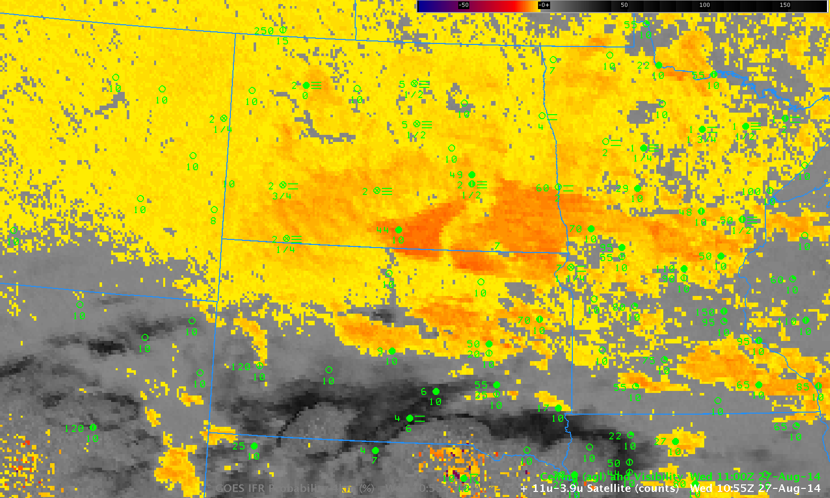
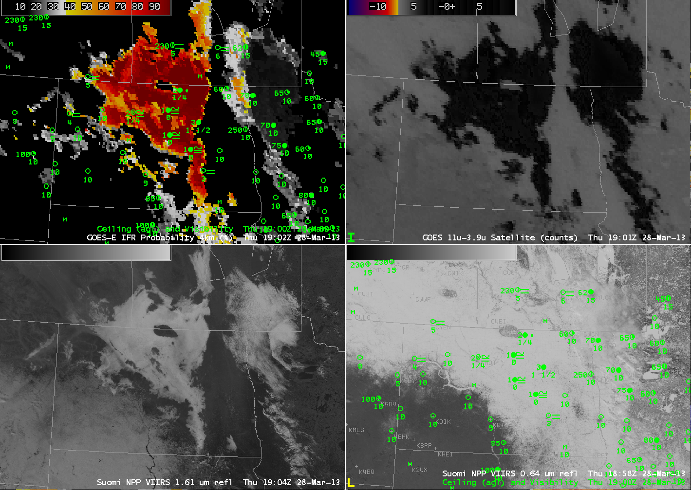
GOES Brightness Temperature Difference (10.7 µm – 3.9 µm) and surface observations of ceilings and visibilities, 1100 UTC, 27 August 2014

GOES data indicated widespread stratus over North Dakota and adjacent states early in the morning on 27 August. The image above demonstrates several difficulties that come with using the brightness temperature difference field to identify regions of reduced ceilings and visibilities. A stratus deck (over eastern Montana) and a fog bank (over central North Dakota) can have a very similar signal in the brightness temperature difference field. Furthermore, regions where ice crystals comprise the clouds (southern South Dakota) show a different signal. Low-level stratus will be invisible to the satellite at night if it is beneath a higher-level cirrus shield.

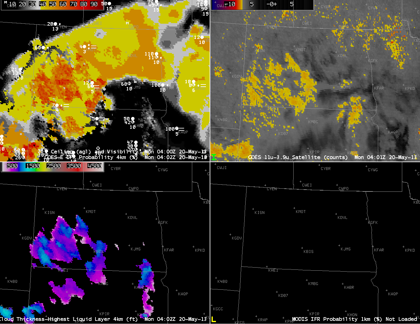
IFR Probabilities for the same time, below, more accurately define where the lowest visibilities and ceilings occur because Rapid Refresh Model data are used to identify regions where part of the lowest layers of the model atmosphere is saturated. If there is saturation below higher clouds (southern South Dakota), then IFR Probabilities are increased. If there is not low-level saturation in the model in regions where low stratus/fog is present, then IFR Probabilities are reduced (eastern Montana).

Note also how the character of the fields changes if satellite data are not used as an IFR Probability predictor. IFR Probabilities in southern South Dakota (where multiple cloud layers are present associated with a convective feature) have a uniform look to them, as they are derived solely from model-based fields. Over North Dakota and Montana, satellite data can be used as a predictor; the individual satellite pixels are obvious. When only model data are used as predictors, the probability is reduced. Thus, the color yellow in a region of model-only prediction (southern South Dakota) should be interpreted differently than the color yellow in a region that uses both model and satellite predictors (North Dakota and Montana).

GOES_IFR_1100UTC_27August2014

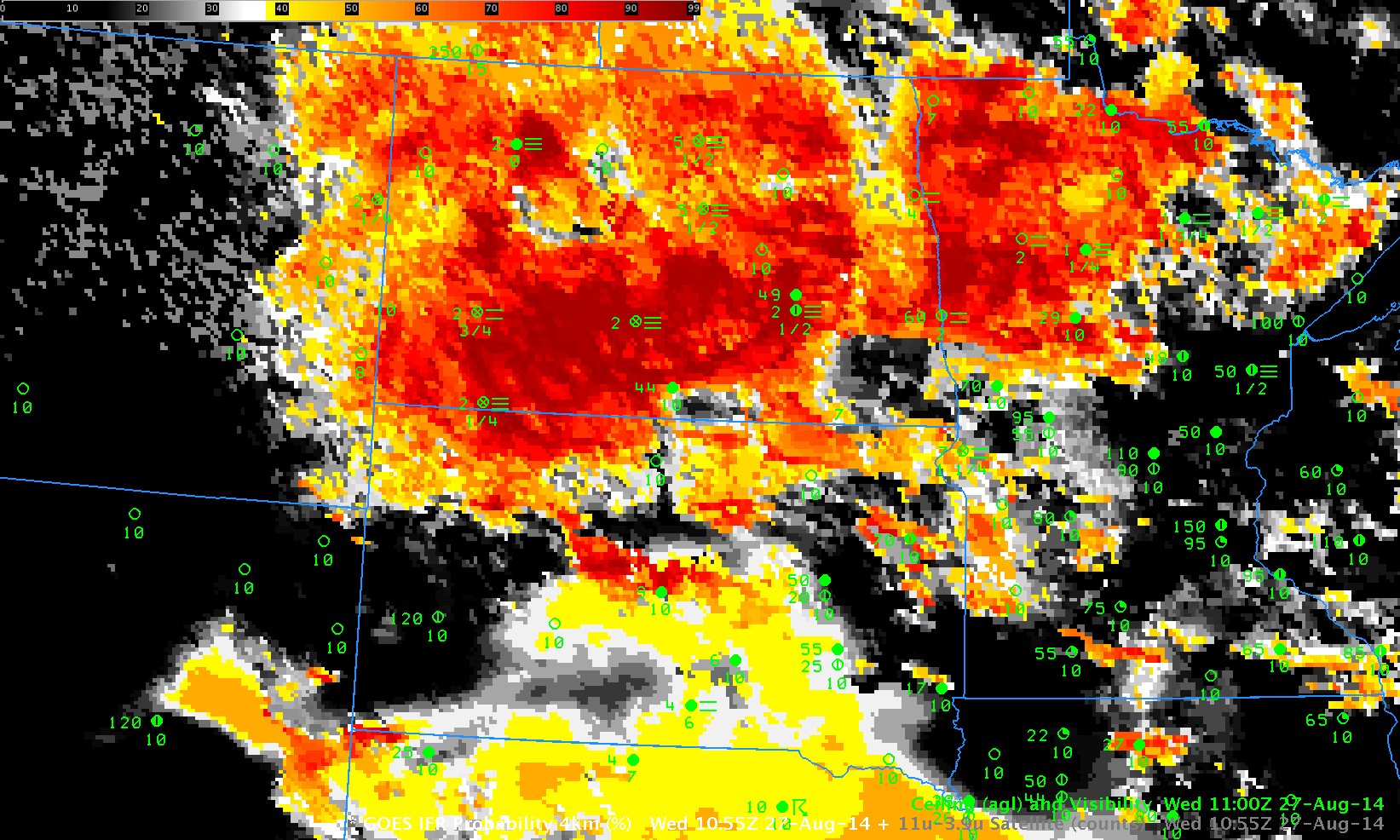
GOES-R IFR Probabilities and observations of ceilings and visibilities, 1100 UTC, 27 August 2014

Stratus and low Stratus over North Dakota

NoDak_0915_25June2014

GOES-based GOES-R IFR Probabilities (Upper Left), GOES-13 Brightness Temperature Difference (10.7µm – 3.9µm) (Upper Right), GOES-R Cloud Thickness (Lower Left), Suomi/NPP Brightness Temperature Difference (11.35µm – 3.74µm) (Lower Right), all times as indicated (Click to enlarge)

A strength of the GOES-R IFR Probability field is that it highlights regions where IFR conditions are occurring and downplays regions where stratus is elevated off the surface, insignificant from an aviation point of view. In the image above, note how stations in the Missouri River valley of central North Dakota (Bismarck, Mercer County) are under a thick stratus deck that is highlighted in the brightness temperature difference fields, but surface ceilings and visibilities are good. IFR Probabilities there are small because the Rapid Refresh Model data does not suggest low-level saturation. Dickinson and Hettinger, over southwestern North Dakota, in contrast, show restricted visibilities (that worsen before sunrise, see below) in a region of higher IFR Probabilities. IFR Probabilities remain low over central North Dakota where visibilities are not restricted.

NoDak_1015_25June2014

GOES-based GOES-R IFR Probabilities (Upper Left), GOES-13 Brightness Temperature Difference (10.7 – 3.9) (Upper Right), GOES-R Cloud Thickness (Lower Left), Suomi/NPP Brightness Temperature Difference (11.35 – 3.74) (Lower Right), all times as indicated (Click to enlarge)

One more example of extreme cold

BTDIFR_20140127_1102toggle

Toggle of GOES-East Brightness Temperature Difference (10.7 µm – 3.9 µm) and GOES-R IFR Probabilities at 1100 UTC, 27 January 2014 (click image to enlarge)

One more example, above, showing the effects of extreme cold on the IFR Probability. IFR Probabilities correctly ignore the regions of low stratus in advance of the extreme cold air over Kansas and over the Ohio River Valley and Great Lakes. However, because of how the pseudo-emissivity is computed (See here also), and because the Rapid Refresh model show saturation in lower levels, regions with extreme cold will show a pixelated signal with noise.

IFR Probabilities in Extreme cold, Continued

GOES_IFR_Reg_11-3.9_Sat_20140106_0231loop


Toggle between GOES-R IFR Probabilities from GOES-13 and GOES-13 Brightness Temperature Difference (10.7 µm – 3.9 µm), with surface observations and ceilings plotted, ~0230 UTC on 6 January 2014. (click image to animate)

The coldest air of the season has plunged into the central part of the US. And as noted before, extreme cold does have an influence on the IFR Probability fields because of how the pseudo-emissivity is computed. Consider this effect of cold on the fields as you interpret them. Note also that in the daytime, when visible imagery can be used to augment the cloud mask, IFR Probabilities are low in very cold airmasses.

IFR Probability fields in extreme cold

GOES_IFR_11-3_20131226_1800toggle

GOES-R IFR Probabilities from GOES-15 with surface ceilings/visibilities and GOES-15 Brightness Temperature Difference (10.7 µm – 3.9 µm) Fields with surface plots at 1800 UTC 26 December 2013 (click image to enlarge)

The image toggle above shows IFR Probability and the Brightness Temperature Difference Field over northern Alaska. Plotted METAR observations show very cold surface temperatures in the -30 to -50 F range. At such cold temperatures, the pseudo-emissivity computation can become noisy because a very small change in 10.7 µm radiance (used to compute the 3.9 µm radiance) can cause a large change in 3.9 µm brightness temperature. (The effect is shown graphically below — a small change in radiance at 3.9 µm leads to a very large temperature change). This noise can lead to a speckled appearance to the IFR probability fields. This effect can also occur in the northern Plains of the United States when surface temperatures dip below zero.

Noise_in_3.9um_ch

Radiance (y-axis) vs. Brightness Temperature (x-axis) for 3.8 µm (left) and 10.7 µm (right)

(update) Below is the IFR Probability in the heart of a Polar Airmass over northwestern Ontario.

GOES_IFR_11-3.9_20131230_1215

GOES-R IFR Probabilities from GOES-13 with surface ceilings/visibilities and GOES-13 Brightness Temperature Difference (10.7 µm – 3.9 µm) Fields with METAR plots at 1215 UTC 29 December 2013 (click image to enlarge)

IFR Conditions in the northern Plains

GOES_IFR_PROB_20131022loop

GOES-13-based GOES-R IFR Probabilities (Upper Left), GOES-13 Brightness Temperature Difference Product (10.7 µm – 3.9 µm) (Upper Right), MODIS-based GOES-R IFR Probabilities (Lower Left), Suomi-NPP Brightness Temperature Difference (11.35 µm – 3.74 µm) (Lower Right), all times as indicated (click image to enlarge)

The animation above shows GOES-R IFR Probabilities highest in a band that stretches mostly north-south from western North Dakota into central South Dakota. IFR conditions are observed under and near this band, for example at Stanley, North Dakota. The occasional MODIS-based IFR Probabilities also suggest that IFR conditions are most likely over the western Dakotas. Both GOES-based and MODIS-based IFR Probability fields de-emphasize the regions of enhanced brightness temperature difference (in both GOES and Suomi-NPP Fields) that exist over western Minnesota and the central and eastern Dakotas. In these regions, mid-level stratus is being detected by the satellite. The Rapid Refresh model is correctly diagnosing the clouds as elevated, and that model information is used to de-emphasize (correctly) the possibility of IFR conditions. IFR and near-IFR conditions also occur over parts of northeast Minnesota into northwest Wisconsin where IFR probabilities are higher.

GOES_IFR_BTD_20131022_0945

Toggle between GOES-13-based GOES-R IFR Probabilities and GOES-13 Brightness Temperature Difference (10.7 µm – 3.9 µm) at 0945 UTC on 22 October (click image to enlarge)

A limitation of the traditional brightness temperature difference product is highlighted above in the toggle between the GOES-R IFR Probability and the Brightness Temperature Difference at 0945 UTC. Mid-level stratus and low stratus/fog look nearly identical in the brightness temperature difference product, but the latter is very significant for aviation. Thus the need to better highlight regions of IFR conditions by using the fused data product that incorporates surface information by way of the Rapid Refresh model.

Lunar illumination is particularly strong at this time (Full moon occurred late last week), so the day/night band on Suomi/NPP gives compelling visible imagery. As with the case with brightness temperature difference products, however, it can be difficult to distinguish between mid-level stratus and low stratus in the Day/Night band. Toggles between the Day/Night band and the Brightness Temperature Difference from Suomi/NPP is at both 0736 and 0918 UTC are below. Work proceeds on incorporating Suomi/NPP data into the GOES-R IFR Probability algorithm.

VIIRS_DNBFOG_20131022_0736

VIIRS_DNBFOG_20131022_0918

Identifying regions of fog underneath multiple cloud layers

GOES-R IFR Probabilities computed from GOES-East (Upper Left), GOES-East Brightness Temperature Difference (10.7 µm- 3.9 µm) (Upper Right), GOES-R Cloud Thickness (Lower Left), GOES-R IFR Probabilities computed from MODIS (Lower Right).  All imagery around 0400 UTC 20 May 2013

When multiple cloud layers are present, the traditional method of detecting fog, the brightness temperature difference between the 10.7 µm and 3.9 µm channels on the GOES Imager, will fail.  For such a configuration of clouds, the GOES-R IFR Probability field will yield information because it also uses information from the Rapid Refresh model to predict whether fog is possible.  The image above contains regions where both model and satellite data are used to compute the IFR probability, and where model data only are used.  How can you differentiate between the two?

Regions over southwest North Dakota are not overlain by high clouds.  In those regions, a strong signal in the brightness temperature difference fields is present.  There is also a north-south oriented signal over extreme southeast North Dakota and northeast South Dakota.  In both of those regions, the Cloud Thickness product is predicting a thickness.  Such a prediction works only when low clouds are visible by the satellite.

The GOES-R IFR Probability field, in the upper left, contains regions where both satellite and model are used (and these mostly overlay the regions where the Cloud Thickness field is present) and where only model data are used (because the satellite signal for low clouds is blocked by mid- and high-level clouds).  The horizontal homogeneity of the field over northeast North Dakota is characteristic of GOES-R IFR Probability fields that are determined largely by model data only.  Compare that to the more pixelated field over southwest North Dakota where Cloud Thickness fields are also computed:  Pixelation is a hallmark of the use of satellite data in the prediction of the IFR Probability.

Hourly evolution of GOES-R IFR Probability (with surface plots of ceiling/visibility) over North Dakota, 2202 UTC 19 May through 1402 UTC 20 May 2013

The GOES-R IFR probability field accurately depicts the region of IFR conditions over northeast North Dakota that is separate from southeast North Dakota where higher ceilings/visibilities are present.  (Consider the observations at Jamestown, ND (KJMS), for example).  As nighttimes progresses, IFR probabilities increase over most of the state.  The switch from daytime predictors (initially) to nighttime predictors is apparent in the 0202 UTC image (the terminator slants southwest to northeast).  The switch back to daytime predictors occurs between the 1102 UTC and 1215 UTC imagery.

Fog Detection over Snow

GOES-R IFR Probabilities computed from GOES-East (Upper Left), GOES Brightness Temperature Difference (10.7 µm- 3.9 µm ) (Upper Right), Suomi/NPP 1.61 µm Reflectivity (Lower Left), Suomi/NPP Visible Imagery (0.64 µm) (Lower Right)

Snow cover in Spring promotes the development of advection fogs when relatively moist air moves over the snowpack and is cooled to its dewpoint, saturating.  But snowcover is also white when viewed from Satellite, and its presence makes the detection of fog areas difficult.  There are several products that can be used to distinguish between white snow and white clouds, and products that can be used to refine further the difference between stratus decks and fogbanks.

In the imagery above, Suomi/NPP 1-km resolution visible (0.64 µm) data in the bottom right figure show a large region of both clouds and snow over the North Dakota and surrounding US States and Canadian Provinces.  It is very difficult to find the cloud edges that are there.  The 1.61 µm imagery from Suomi/NPP is very helpful in screening out imagery of snow on the ground.  Water clouds are far more effective at reflecting radiation at wavelengths around 1.61 µm than snow or ice (snow and ice both strongly absorb radiation at that wavelength).  Thus, in the bottom left figure, the 1.61 µm reflectivity detected by Suomi/NPP, areas of snow appear dark and areas of water-based clouds are white.  This tells you where water clouds exist, but nothing about how high above the surface those water clouds are.  The brightness temperature difference product from GOES (10.7 µm – 3.9 µm) also highlights in dark regions of water-based clouds, but as with the 1.61 µm reflectivity does not give information about cloud bases.

The GOES-R Fog/Low Stratus IFR Probability neatly distinguished between the stratus deck over western Minnesota (that is not accompanied by IFR conditions at the surface) from the cloudy region over central and northern North Dakota that is accompanied by IFR conditions at the surface, as shown in the plotted observations.  (Thanks to Chad Gravelle for noticing this case today!)

Multiple Cloud Layers/High Clouds over Fog

GOES-R IFR Probabilities computed from GOES-East (Upper Left), GOES-East Brightness Temperature Difference (10.7 µm – 3.9 µm) (Upper Right), GOES-R Cloud Thickness of highest liquid water layer (Lower Left), GOES-East Water Vapor (6.7 µm) (Lower Right)

It’s very common in late Winter and early Spring to have a cirrus shield over a region of dense advection fog.  The water vapor imagery, above, shows the cirrus associated with a developing warm conveyor belt over the central part of the USA.  Note how the cirrus signal also shows up in the brightness temperature difference field, and the emissivity properties of ice clouds differ strongly from those of water-based clouds (that in the enhancement in the upper right are orange versus black for ice clouds).  The presence of cirrus also precludes computation of GOES-R cloud thickness, as shown in the lower left imagery.

GOES-R IFR probabilities allow for the identification of regions of low clouds/fog even underneath the high clouds.  Note over Michigan the relatively high probabilities.  The probabilities are generated using only model-based predictors (because the satellite algorithm sees only the high clouds so satellite predictors are very small or missing).   The 1000 and 1300 UTC imagery, below, shows widespread IFR conditions underneath cirrus over Michigan and surrounding states.  IFR conditions are generally present in regions where the IFR probabilities are high.  Ceilings/visibilities do not meet IFR criteria over Western Illinois where IFR Probabilities are much lower.

As above, but centered over Michigan

Advection Fog in the Midwest

GOES-R IFR Probabilities from GOES-East, hourly from 00:15 through 13:15 on 28 January 2013, with surface visibilities and ceilings.

Warm and moist air streaming north from the southern Plains has encountered the cold (and in some places) snow-covered ground.  This is a time-honored recipe for advection fog, and the GOES-R IFR Probabilities fields, above, neatly capture the horizontal extent of the visibility restrictions overnight.  The highest IFR Probabilities occur in regions where both Satellite Predictors and Model-based predictors are high.  Note, for example, the somewhat lower probabilities that develop over Nebraska at the end of the animation.  This is a region where higher clouds are moving in.

GOES-R IFR Probabilities (Upper Left), GOES-East Brightness Temperature Difference (10.7 µm – 3.9 µm) (Upper Right), GOES-R Cloud Thickness (Lower Left), GOES-East 10.7 µm Brightness Temperature (Lower Right)

Note how the Cloud Thickness product is not computed where the higher clouds are moving in.  The product is computed only where single layer clouds are present in non-twilight conditions.  Twilight conditions are present in the eastern half of the final image, at 1315 UTC.  When radiation fog is present (rather than advection fog in this case), the last cloud thickness before twilight conditions can be used to estimate dissipation time using this chart.

GOES-R IFR Probabilities (Upper Left), GOES-East Brightness Temperature Difference (10.7 µm – 3.9 µm) (Upper Right), GOES-R Cloud Thickness (Lower Left), GOES-East Visible Imagery (0.62 µm) (Lower Right)

Holes in the advection fog developed around 1700 UTC.