 |
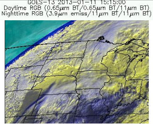
| False color image of a winter storm system moving across the upper Midwest U.S. on 11 January 2013. |
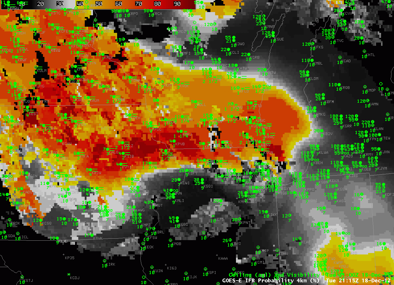
A strong winter storm system moved over the upper Midwest on 11 January 2013 bringing heavy snow to the Dakotas. Rain and warm air moved in over the mostly snow covered areas of eastern Nebraska, Minnesota, Iowa, Wisconsin and northern Illinois resulting in a large area of locally dense fog. GOES-R IFR probabilities were used to monitor the large-scale event as it moved over the Upper Midwest U.S.
Due to a large amount of overlaying clouds a satellite only product such as the traditionally-used 11-3.9 micron Brightness Temperature Difference (BTD) only sees the top cloud layer and therefore can not detect fog/low stratus (FLS) beneath. The GOES-R IFR probabilities, however, combine both satellite and mesoscale NWP model data to create a blended product that can estimate the probability that IFR conditions are present even where overlaying clouds obscure all or part of the scene. This animation of the weather system shows that the traditional 11-3.9 micron BTD product only detects a small portion of the fog event, confirmed by the surface observations of ceiling and visibility. The GOES-R FLS product provides relatively high probabilities (>50%) that IFR conditions are present over the entire extent of the fog event with significantly high probabilities (>90%) when satellite data is useful.
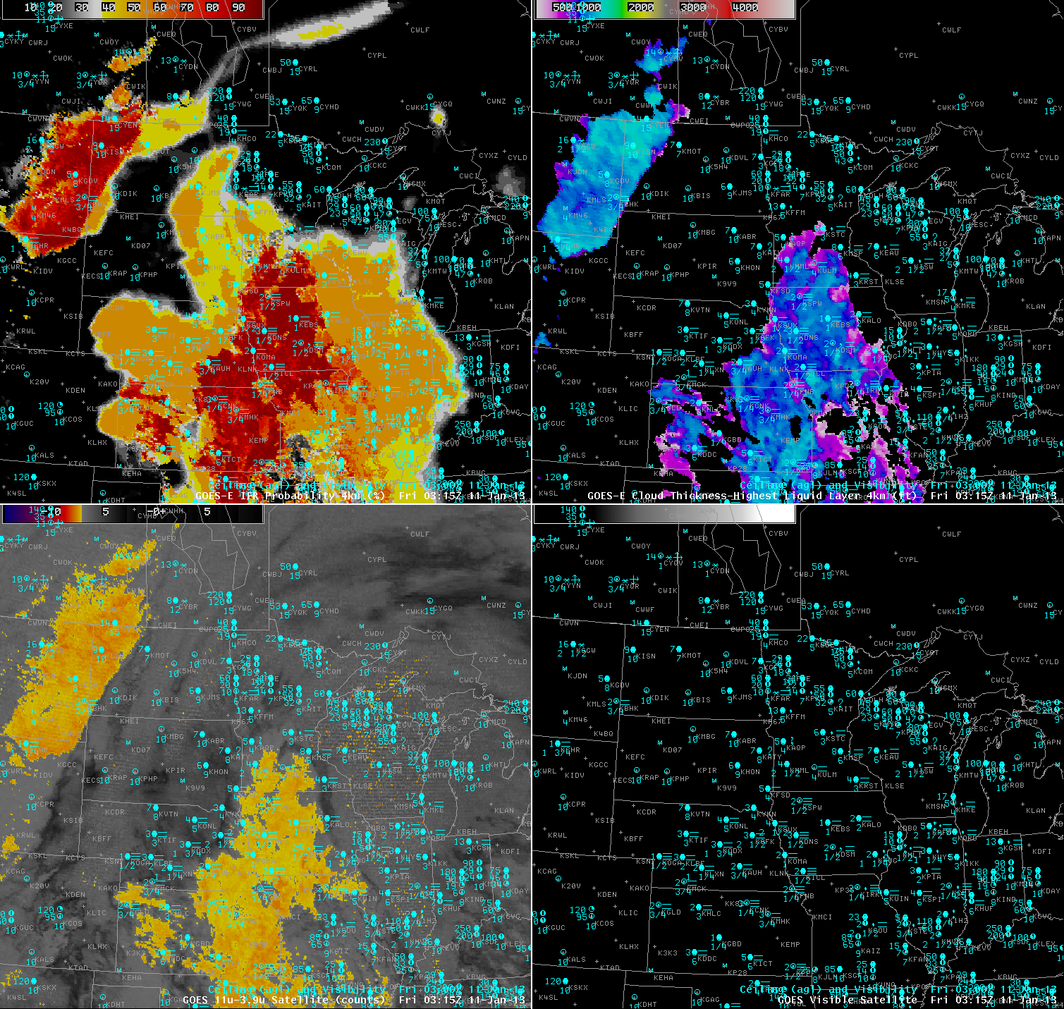 |
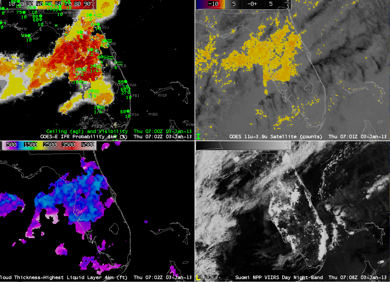
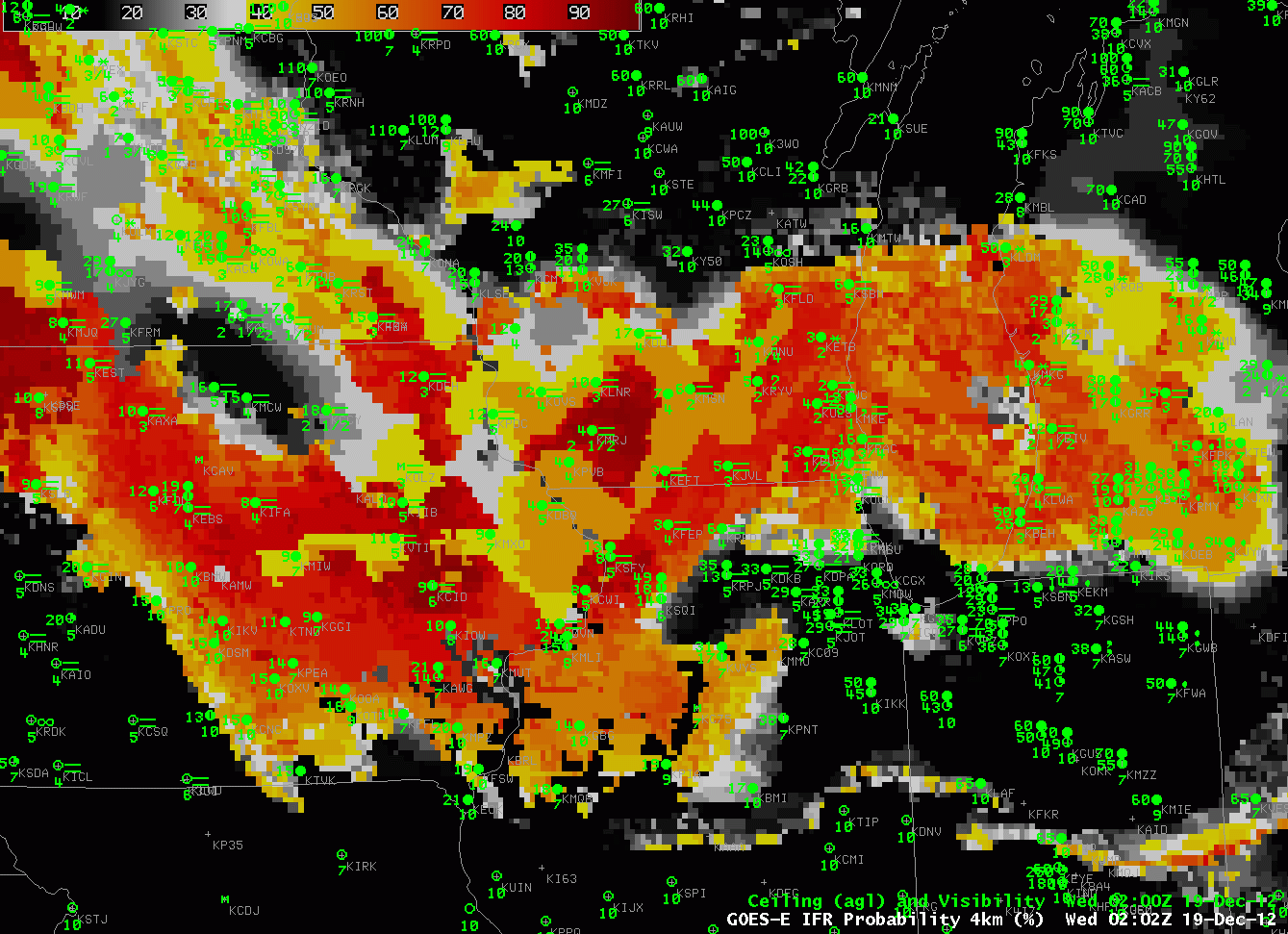
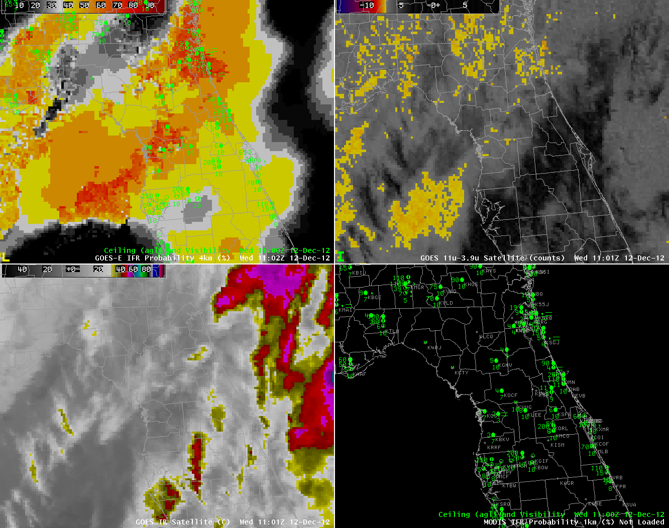
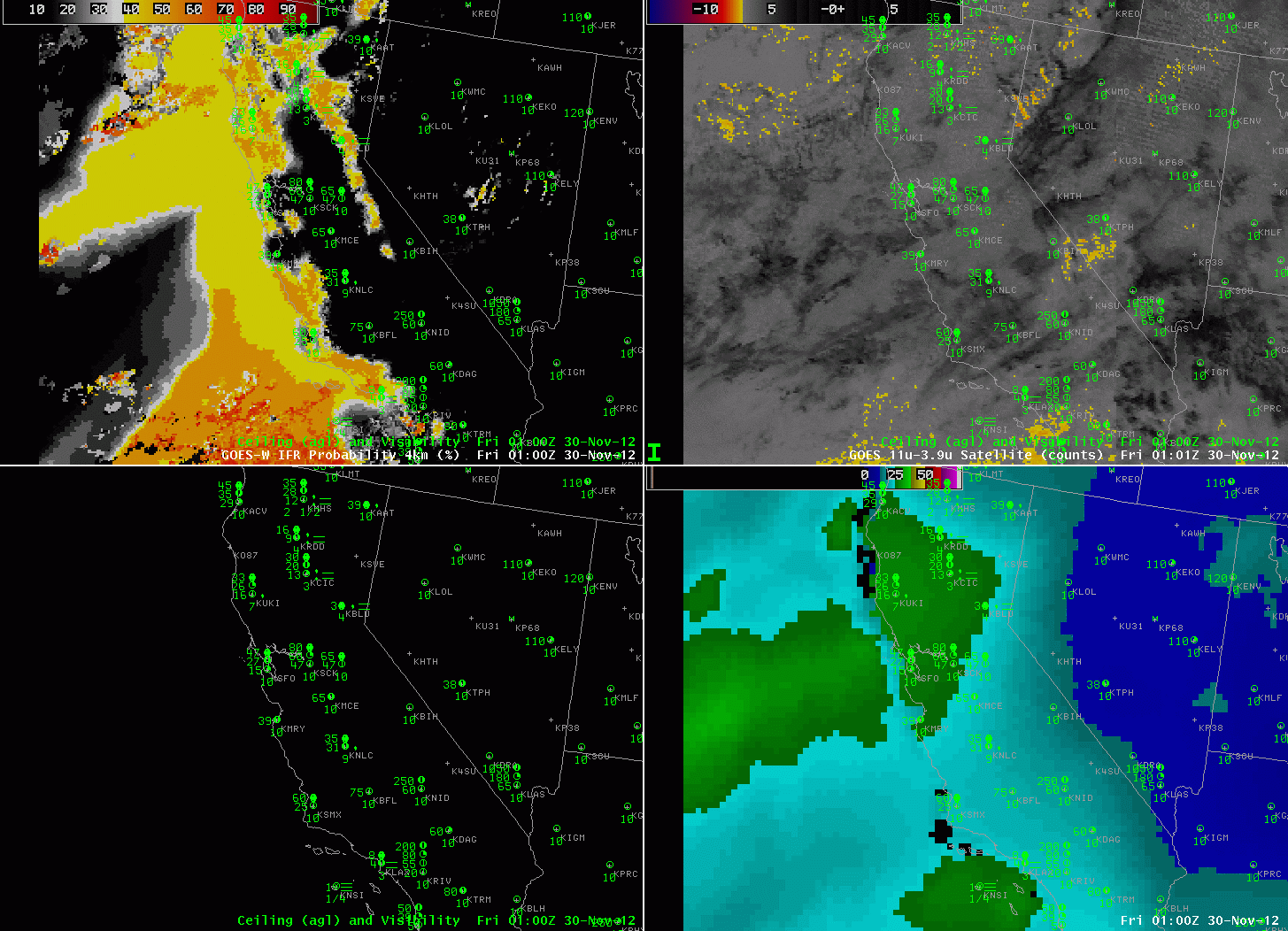
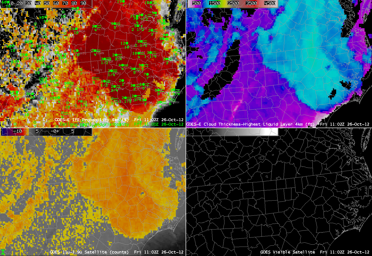
| GOES-R IFR probabilities (Upper Left), GOES-R Cloud Thickness (Upper Right), GOES-East Brightness Temperature Difference (10.7µm – 3.9µm) (Lower Left) and GOES-East Visible Satellite Imagery (Lower Right) on 11 January 2013. Surface observations of ceiling (100’s of ft) and visibility (miles) are shown in blue. |
In the scene above the large change in probability seen in the GOES-R IFR product is a direct result of where the overlaying clouds obstruct the view of the lower clouds from the satellite. Where the satellite is able to see the low level clouds both satellite and model information are combined to determine the probability that IFR conditions are present. For this scene a strong satellite component and strong model component result in extremely high probabilities (>90%) that provide high confidence that IFR conditions are present over parts of the region. In areas where the overlaying clouds obstruct the satellite view only model data is used to determine the IFR probabilities. Without a strong satellite component the resulting probabilities are lower, however, they are still relatively high (>50%) and when used in conjunction with surface observations also provide high confidence that IFR conditions are present. The IFR probabilities show the extent of the fog over central Nebraska, southern Wisconsin and Illinois better than the traditional BTD product with very little false detection (high probabilities where surface obs do not indicate IFR conditions). Looking over the Dakotas and Nebraska the GOES-R IFR probabilities closely match the surface observations with relatively high probabilities over all of Nebraska and the eastern Dakotas where IFR conditions are present and very low probabilities in central N. Dakota and western S. Dakota where surface obs indicate VFR conditions.
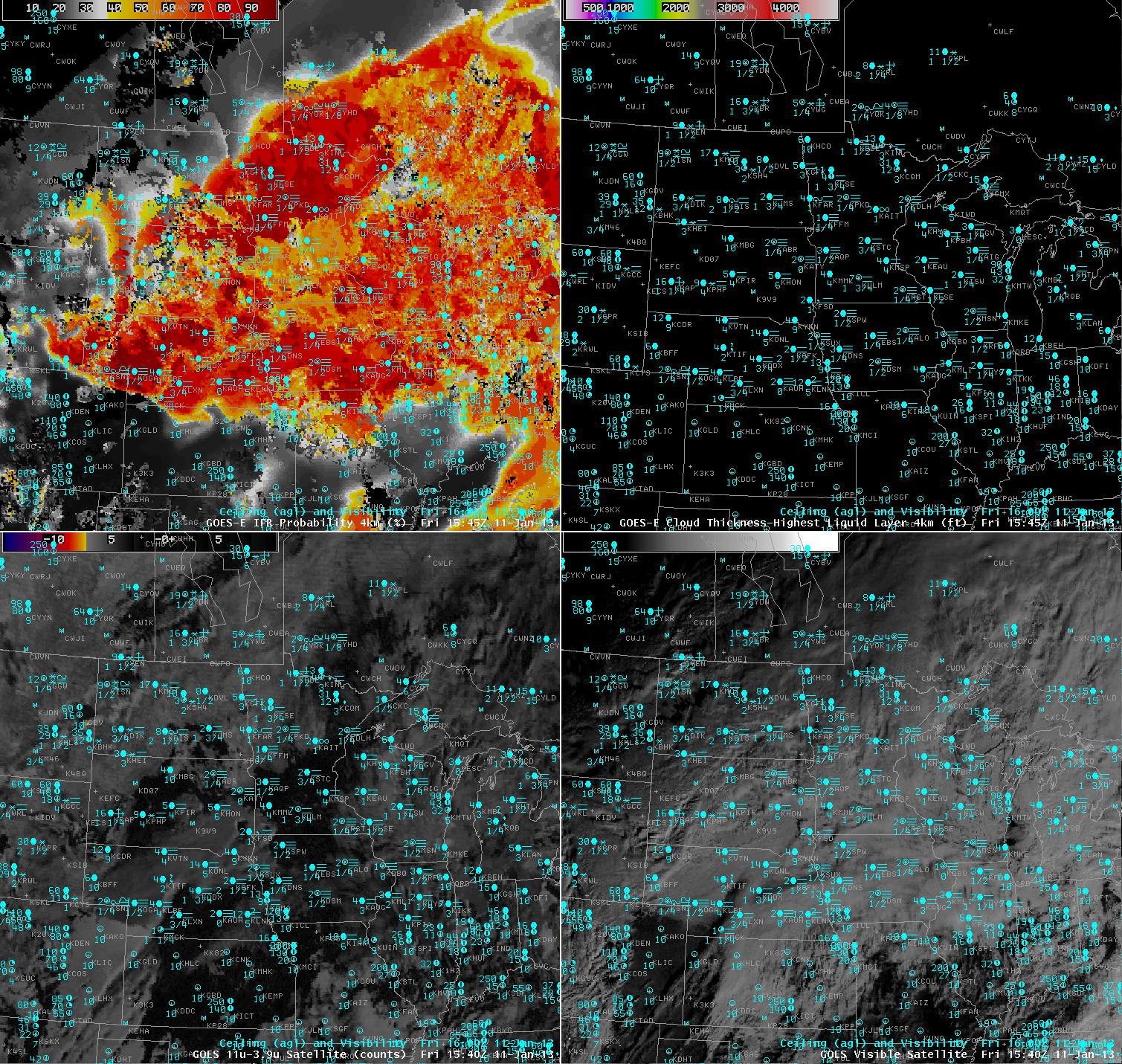 |
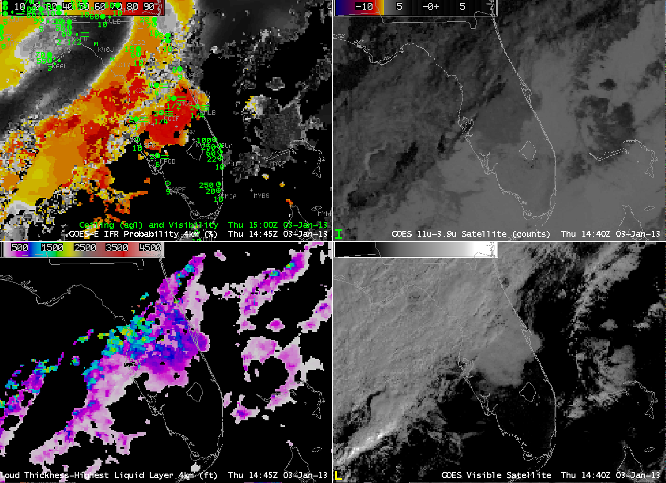
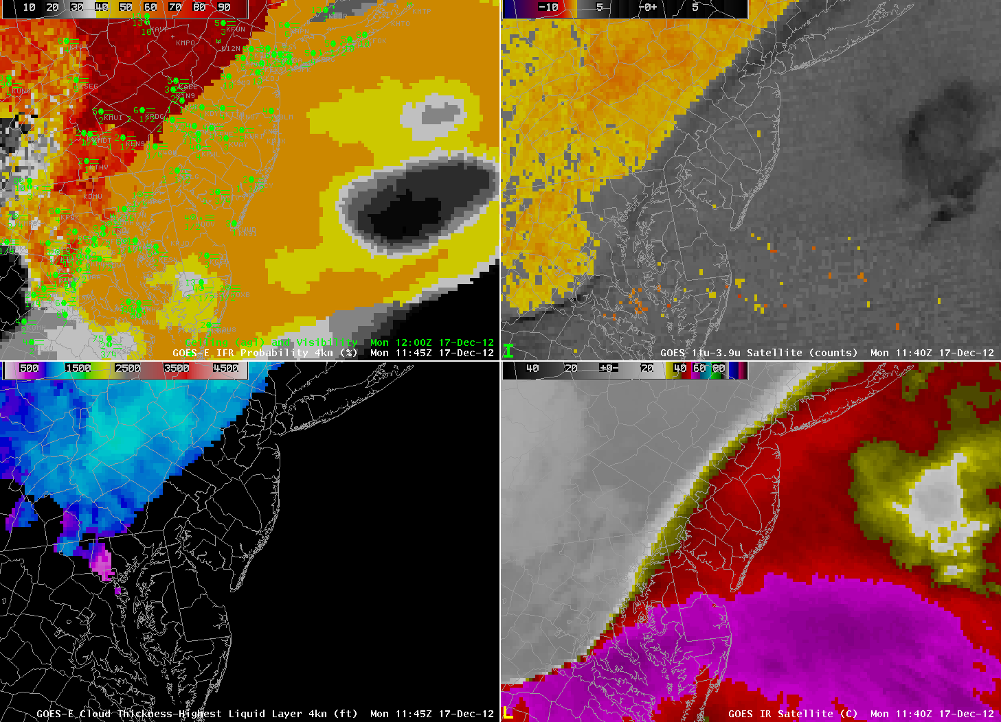
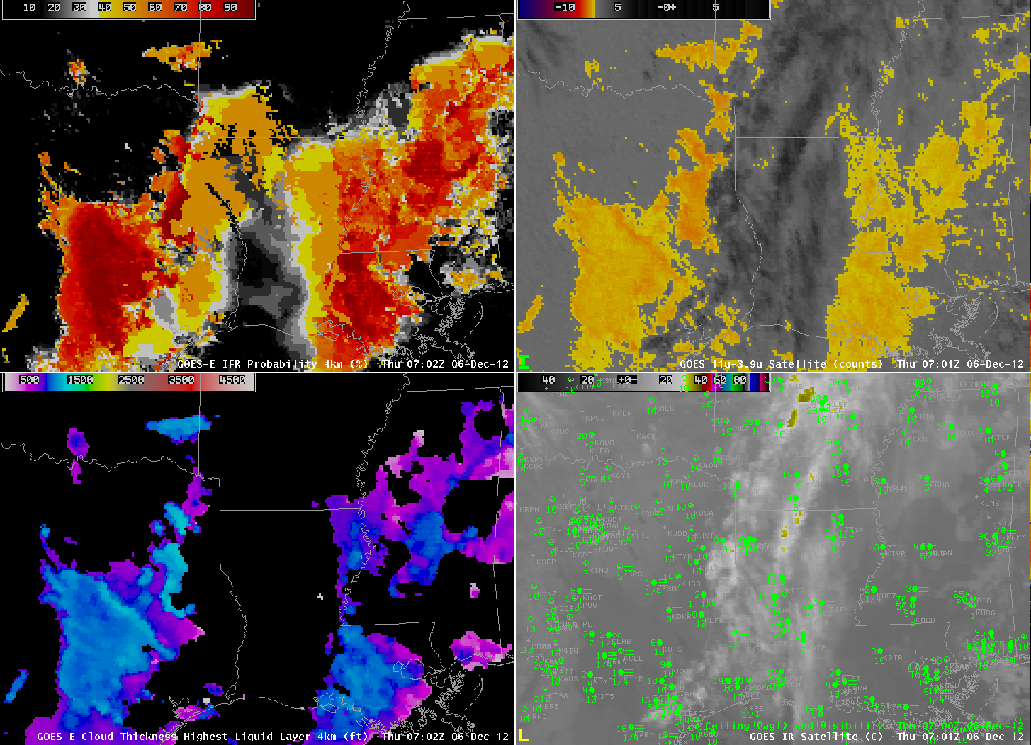
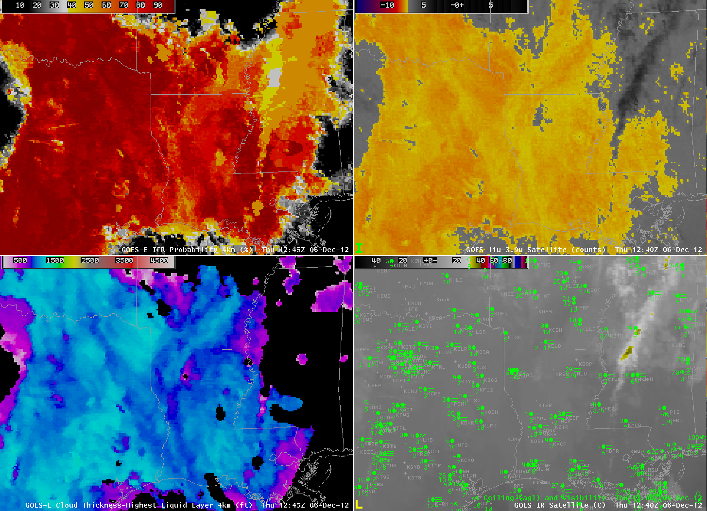
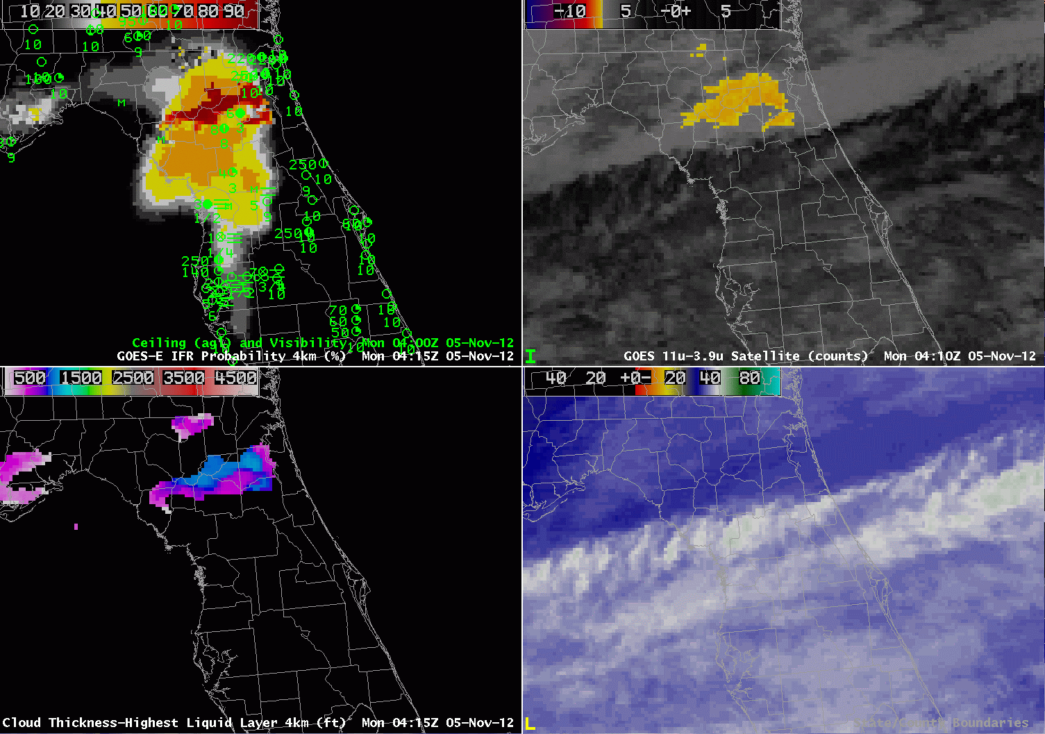
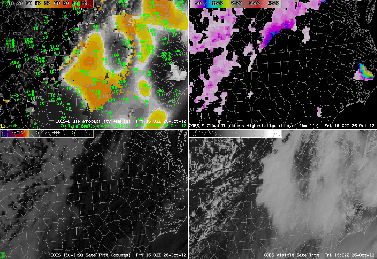
| GOES-R IFR probabilities (Upper Left), GOES-R Cloud Thickness (Upper Right), GOES-East Brightness Temperature Difference (10.7µm – 3.9µm) (Lower Left) and GOES-East Visible Satellite Imagery (Lower Right) on 11 January 2013. Surface observations of ceiling (100’s of ft) and visibility (miles) are shown in blue. |
The traditional BTD product is mostly a nighttime only product as solar contamination in the 3.9 micron channel during the day makes it much more difficult to use. As daylight approaches the scene from 11 January 2013 the traditional BTD product appears to drop out. The GOES-R IFR product has no such issues and works smoothly through the night-to-day transition with consistently high probabilities accurately showing the full extent of the area of fog that continued through the rest of the afternoon.

