Category Archives: MODIS

The Terminator

GOES-R IFR Probabilities near sunrise on 27 July 2012

The loop above demonstrates an artifact of the GOES-R IFR probabilities that occurs due to the terminator.  Note how values within the circled region are constant for the last three images.   When the solar zenith angle is between 85-90 degrees there is a stabilizing temporal aspect to the algorithm. In these 5 degrees (just after sunrise), the last nighttime satellite parameters from an angle >90 degrees are kept and used (and re-used) because the visible channels are not reliable at such high solar zenith angles. Current Rapid Refresh model information is used, but if the model data doesn’t vary greatly over this timeframe then it is likely that the same information will be used for the Bayesian model, thus resulting in the same probability values. This approach reduces significant artifacts in the terminator region where FLS detection is complicated by a low sun angle and the attendant rapid changes in reflectivity.

MODIS-based IFR probabilities at 0835 UTC.  Because western Kentucky is at the edge of the MODIS scan, some bow-tie correction artifacts are present.  Nevertheless, high probabilities nicely correspond to observations of reduced visibilities/ceilings.

Note that this is occurring in a region of fog as evidenced by the MODIS-based IFR probabilities at 0900 UTC (above).  The image at 1215 UTC (below), 30 minutes after the end of the animation above, shows how the IFR probabilities have evolved as the sun rises.

GOES-R IFR Probabilities as computed from GOES-East information, 1215 UTC on 27 July 2012.

Spatial and Temporal Resolution

GOES-R IFR Probabilities computed from MODIS data (upper left) and from GOES-East data (lower left);  Ceiling and visibility observations (upper right) and 10.7-micrometer brightness temperatures from GOES-East (lower right)

GOES-R IFR Probabilities can be computed using GOES-East Imager data (the Imager has 5 radiometric channels), with a nominal resolution of 4 kilometers at the sub-satellite point (The Equator, at 75 degrees W for GOES-East;  Actual resolution in the upper midwest is closer to 5 or 6 kilometers).  IFR Probabilities can also be computed using MODIS data from Terra or Aqua;  the MODIS instrument yields information at 36 different radiometric channels, with a nadir resolution of 1 km.  Thus, small-scale features, such as river valleys, or ridge-tops, are far more likely to be visible in the data.  However, MODIS data are available infrequently because Terra and Aqua are polar orbiters, and each satellite passes over a location in the upper Midwest only 2 times daily.

The strength of GOES-R IFR imagery is its temporal resolution.  Routine imaging every 15 minutes is typical, and that allows observations of fog development, as shown in the loop below.  The increase in GOES-R IFR probabilities alerts the forecaster to a region of interest, where more vigilant monitoring of sky conditions may be warranted.  The surface observations do show decreasing visibilities and ceilings where the IFR probabilities are increasing;  that is, the IFR probabilities and actual observations are consistent.

GOES-R IFR Probabilities computed using GOES-East imager data and surface observations of visibility and ceiling from 0400 UTC to 1400 UTC on 26 July 2012.

The ABI (Advanced Baseline Imager) on GOES-R will have twice the resolution of the current GOES Imager (that is, 2 kilometer for infrared channels at the subsatellite point) and higher temporal resolution as well.

Isolated Fog/Low Stratus in Texas

GOES-R IFR Probabilities computed using MODIS data (upper left), MODIS Brightness Temperature Difference (the ‘traditional’ Fog Product) (upper right), Lowest 1km Relative Humidity from the NAM (lower left), MODIS IR Window Channel (lower right)

The MODIS-based GOES-R IFR probability image, above, showed a region of high probabilities of IFR over Bandera and Real Counties in Texas west of San Antonio.  This signal is driven by the brightness temperature difference (shown, upper right) and the relative humidity in the Rapid Refresh.  The NAM relative humidity is shown in the lower left image, and the signal in the GOES-R IFR field suggests the RAP relative humidity is similar.  Note how the brightness temperature difference signal farther west in the image does not lead to a signal in the IFR Probabilities;  model relative humidities there are lower.

Does the high probability of IFR signal verify?  In other words, when you see an isolated signal like this, how much credence can you give it?  Hondo, TX (HDO), just southeast of the higher IFR probabilities, does not show IFR conditions.  How do things evolve with time?  GOES-based imagery, below, show the expansion of the IFR probabilities from 0800 UTC, the approximate time of the MODIS pass, above, to 1030 UTC.  The expansion is typical of what would occur with radiational fog formation overnight.  By 1100 UTC, ceilings at Hondo (HDO) and Rocksprings (ECU) are near IFR conditions.  It appears that the IFR probability signal is correctly diagnosing the slow development of a  fog/stratus deck.

GOES-R IFR Probabilities (Upper left), Ceilings and Visibility plotted over GOES-R Cloud Thickness (upper right), GOES-East enhanced Window Channel brightness temperature (bottom left), GOES-East Brightness Temperature Difference (bottom right) from 0800 UTC

GOES-R IFR Probabilities (Upper left), Ceilings and Visibility plotted over GOES-R Cloud Thickness (upper right), GOES-East enhanced Window Channel brightness temperature (bottom left), GOES-East Brightness Temperature Difference (bottom right) from 1030-1100 UTC

There was a fortuitous pass of the Suomi/NPP satellite over this region as the fog/low stratus developed.  Does that satellite give any more information about the presence of fog?  The loop below toggles between the GOES-R IFR probability from GOES-East data and the Day/Night Band from VIIRS.  Because the Moon is nearly new, very little moonlight is illuminating the cloud field so it is difficult to determine if fog is actually present at 0832 UTC over the region.  The parts of the counties over which the fog is developing are sparsely populated, so there are no city lights from which to glean information.

Pacific NW Fog Event

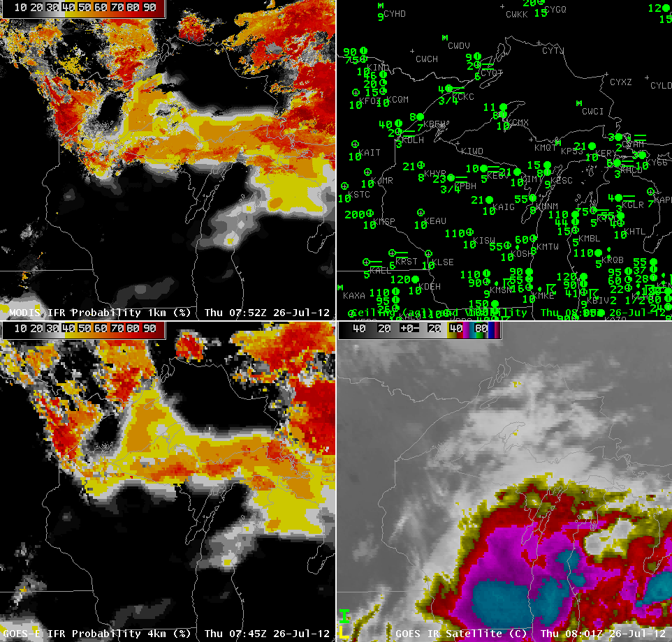
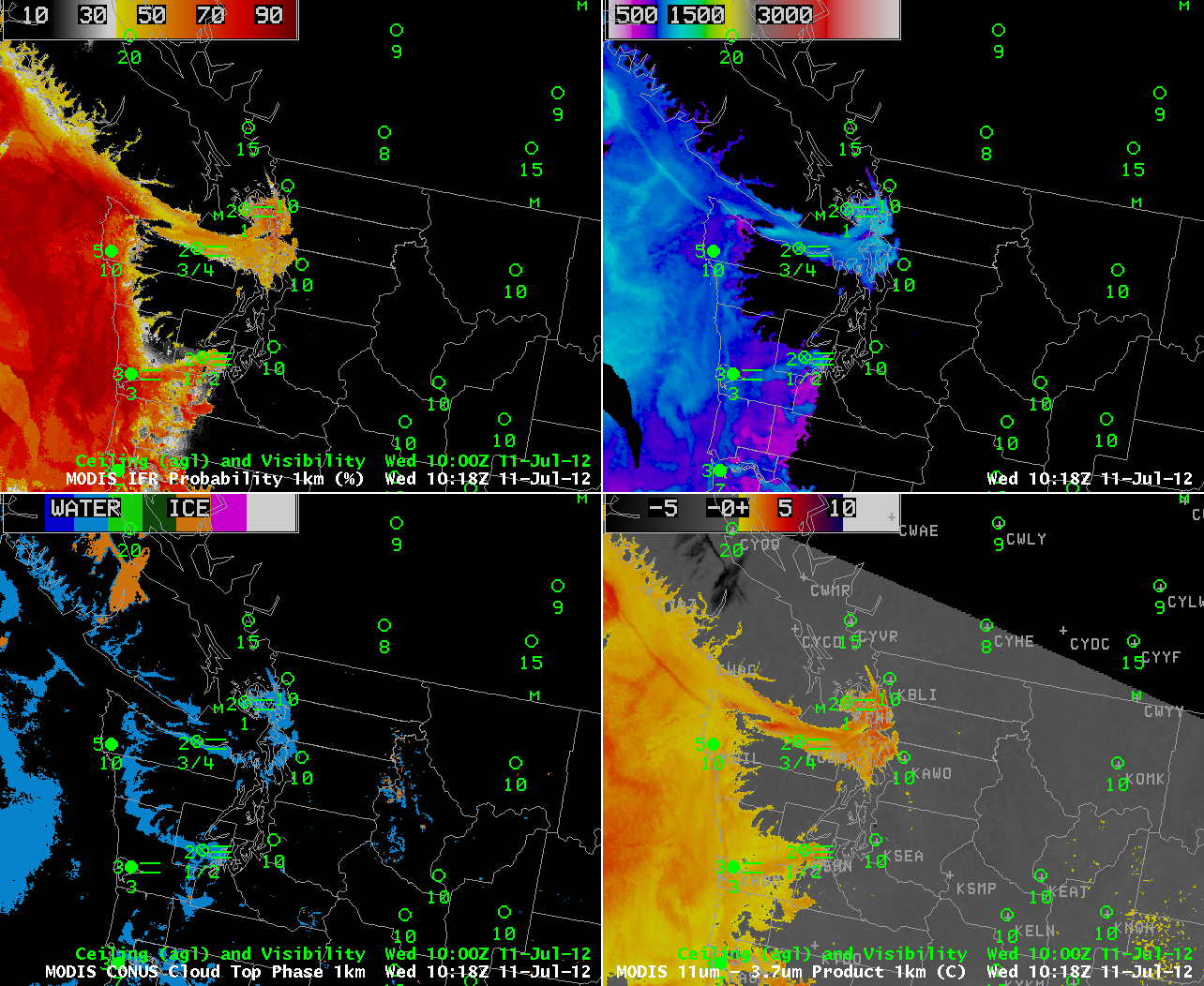
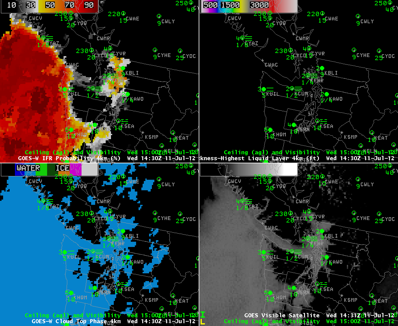
The image above shows IFR probabilities (upper left), Cloud depth (upper right), Cloud type (lower left) and enhanced brightness temperature differences (11 microns – 3.7 microns) for a Puget Sound Fog Event on 11 July 2012.  Heightened IFR probabilities occur where surface observations show IFR conditions are present.

Cloud depths at KUIL, on the coast of Washington are around 800 feet.   The sounding from 72797, below, shows a saturated region between 962 mb and 949 mb.  This is equivalent to a depth (using the hypsometric equation and a mean Temperature in the layer of 13.4 C) of 114 m.  If the cloud bases extend down to 980 mb — a possibility — then the layer depth would be about 270 m.  Note that the MODIS imagery is not at 1200 UTC, the time of the sounding.

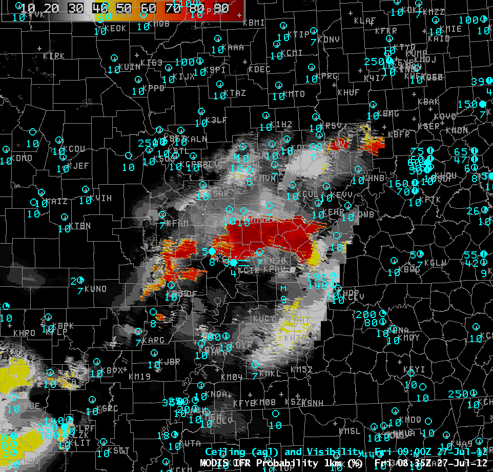
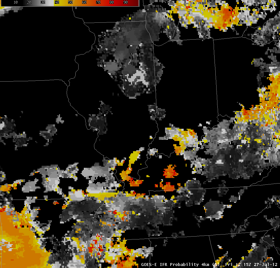
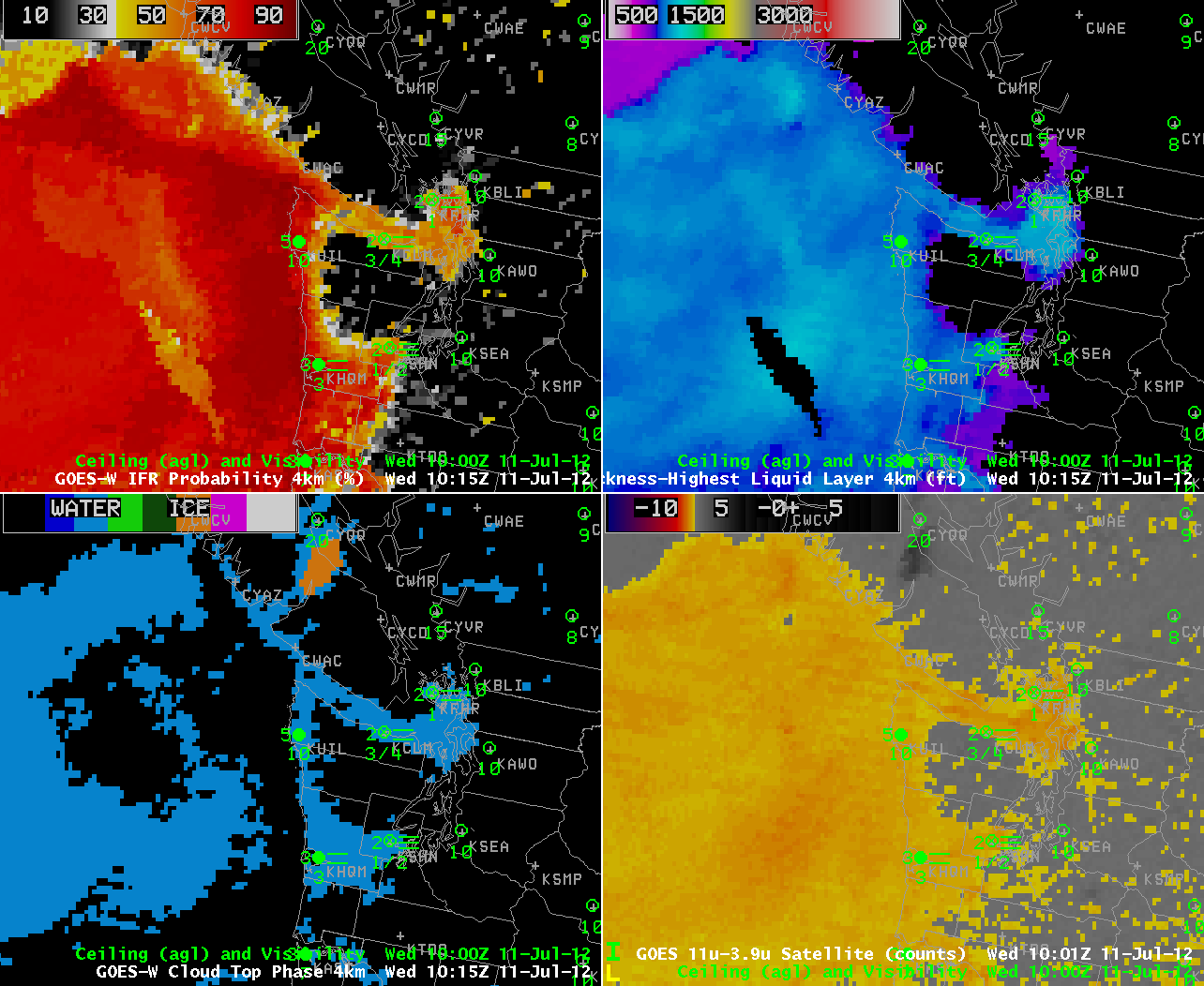
GOES data can also be used to produce Fog/Low stratus products.  The GOES Image from the same time, below, shows similar patterns as the MODIS imagery, with the expected differences due to GOES’s inferior resolution.  In particular, GOES has difficulties detecting small spatial variability in fog that arises due to river valleys.  Note also that the cloud depth at 1015 UTC from GOES shows good agreement with the MODIS product:  values are around 900-1000 feet.  These values persist through 1200 UTC (the nominal time of the sounding) and beyond.

Note in the Cloud Phase product at night the difficulties inherent in detecting low water clouds over the ocean.  Those regions off the coast of Washington are not in fact clear, and both the brightness temperature difference and GOES-R Fog products correctly show fog or low stratus in those areas.

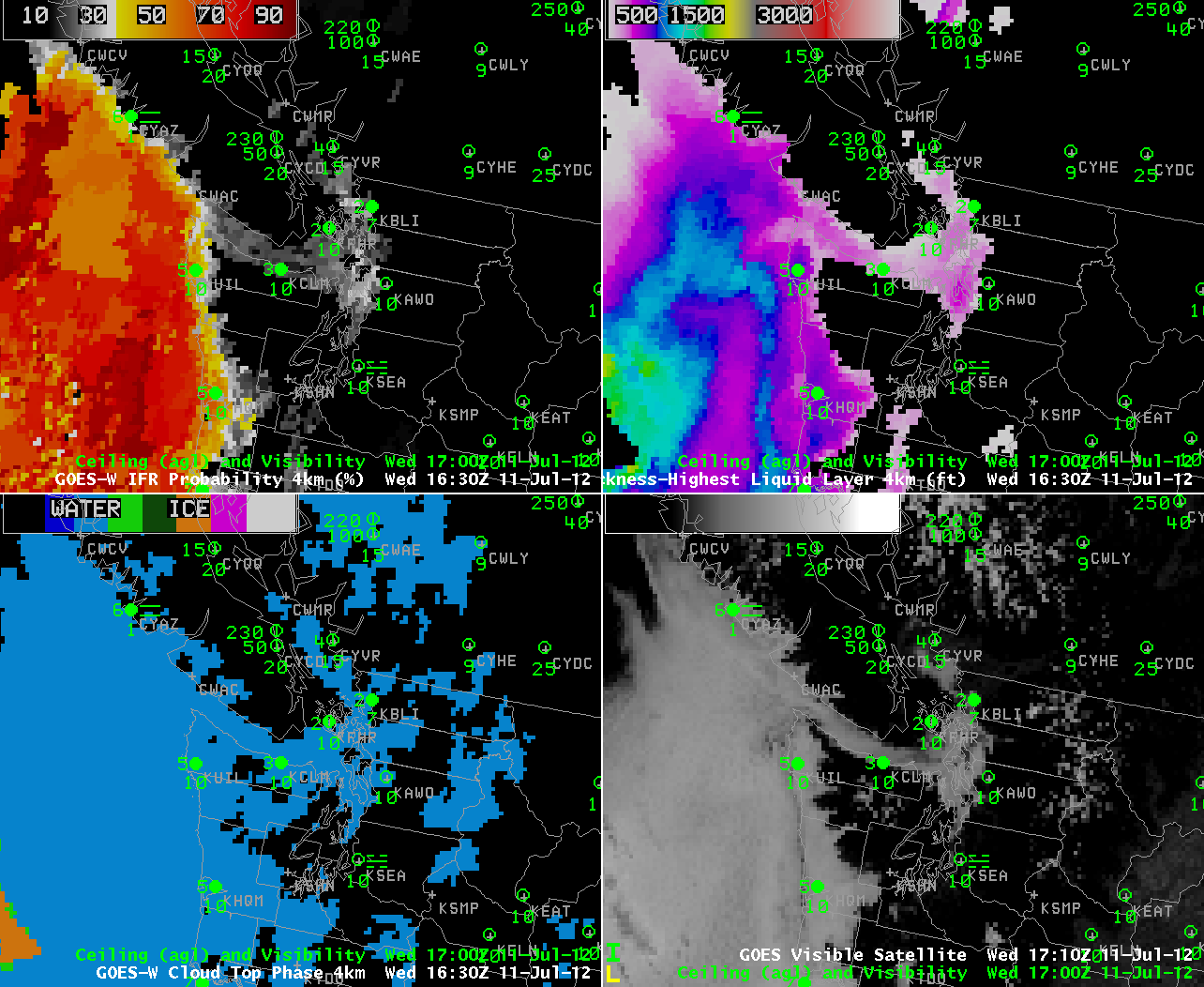
After sunrise, above (the images at 1430/1500 and 1630/1700 UTC), a couple of things change and are noteworthy.  First, the Cloud Top Phase product becomes more complete over the ocean as visible data is incorporated into the algorithm.  Incorporation of visible data reduces Fog/Low Stratus probabilities over the Puget Sound however, even as visible imagery shows persistent clouds there, and adjacent observations (KCLM/Pt. Angeles, for example) show continued IFR conditions.  This may be related to non-uniformity in the horizontal in the visible imagery.