Category Archives: Midwest

Satellite and Model Predictors of Fog

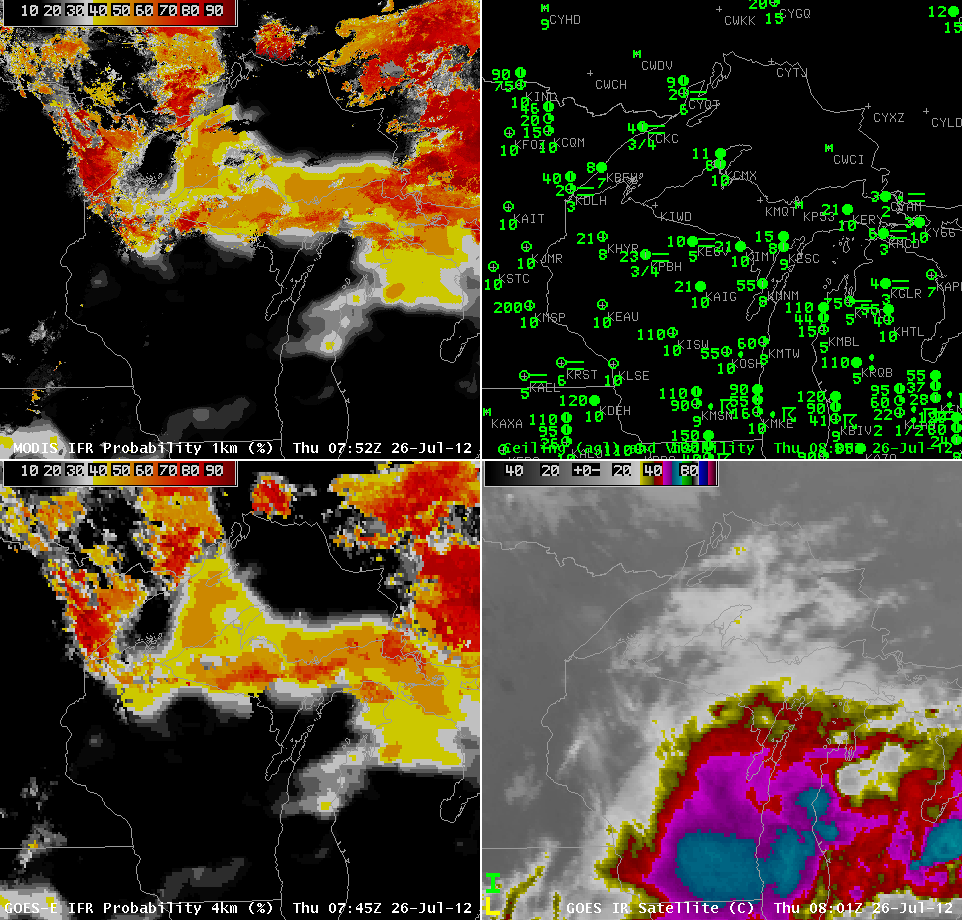
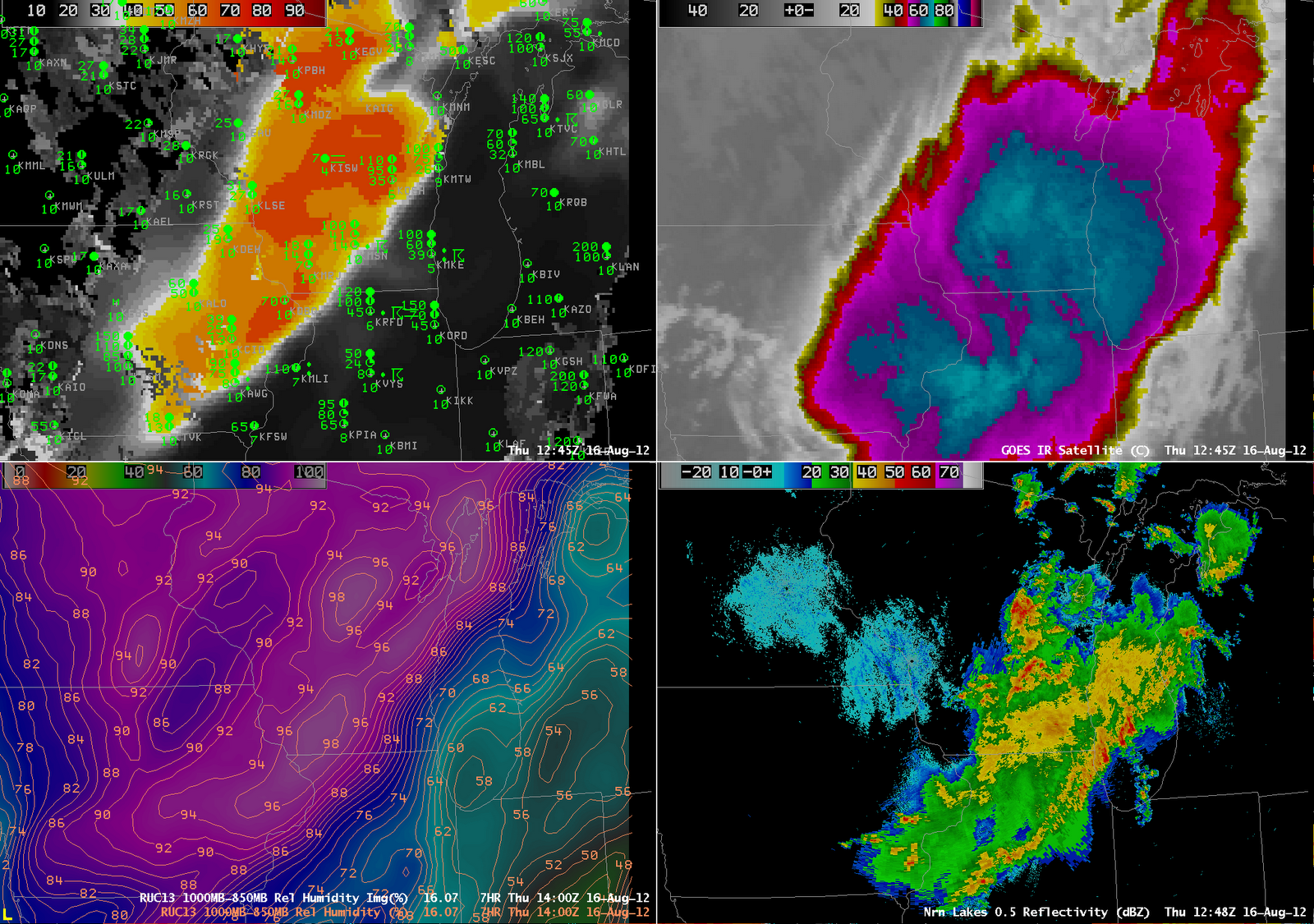
GOES-R IFR Probabilities (Upper left), Enhanced GOES-East 10.7 micrometer imagery (Upper right), Rapid Refresh Mean Relative Humidity (1000-850 mb) (Lower left), Composite Radar Reflectivity (Lower right).  Times as indicated.

A large convective system moved over Wisconsin during the morning of 16 August 2012 and it illustrates the importance of fused data in diagnosing IFR conditions.  The deep convective cloud precludes any satellite detection of low water-based clouds, so the traditional method of detecting fog/low stratus (the brightness temperature difference between 10.7 and 3.9 micrometers) cannot be used.  In this case, model data, in the form of Rapid Refresh Relative Humidity, is used to fill in regions where satellite predictors cannot help.  Note the observation of IFR conditions at Wisconsin Rapids (KISW);  this is a region of very high model relative humidity.  Model relative humidity is just as high over south-central Minnesota;  in that region, however, satellite predictors do exist, and they do not suggest fog/low clouds, so the IFR probability there is comparitively lower.

The character of the IFR probability field is much less pixelated in regions where model data only are used as predictors.  When satellite data and model data are used, as over northwest Wisconsin, for example, the pixelated nature of the satellite data becomes apparent.

Resolution and River Valleys

Animation of GOES-R IFR probabilities (upper left), GOES-R Cloud Thickness (upper right), GOES-East Brightness Temperature Differences (lower left), and Visible Imagery (lower right), from 0400 through 1400 UTC on 6 August 2012

River Valleys — sources of moisture — are nearly sub-pixel scale in GOES-East imagery.  Thus, any signal that develops in a river valley will likely take time to appear, and an example of that occurred over the upper Midwest on the morning of August 6th.  The signal develops along the river starting around 0800 — 0900 UTC (LaCrosse, WI, starts to report visibility and ceiling obstructions at 1000 UTC).  There are several interesting aspects in the loop.

GOES-R IFR probabilities (upper left), GOES-R Cloud Thickness (upper right), GOES-East Brightness Temperature Differences (lower left), and Visible Imagery (lower right), at 0502 UTC on 6 August 2012

The imagery at 0502 UTC (above) shows the result of stray light contamination on the brightness temperature difference field (lower left), but this increase in signal over the Plains is ephemeral, and it is gone in 15 minutes.  There is also an increase in the brightness temperature difference signal over the Plains as sunrise approaches.

GOES-R IFR probabilities (upper left), GOES-R Cloud Thickness (upper right), GOES-East Brightness Temperature Differences (lower left), and Visible Imagery (lower right), at 0915 UTC on 6 August 2012

By 0915 UTC, the GOES-R IFR probabilities have increased slightly along the Wisconsin River in southwest Wisconsin, as has the brightness temperature difference signal (although that signal has increased elsewhere as well where the GOES-R IFR probabilities remain low).  Compare the (relatively) low-resolution GOES-based imagery to the higher resolution Suomi/NPP resolution discussed here.  Note also how the GOES-R IFR probability product correctly suppresses the IFR probabilities over Iowa and Missouri where observations show no obstructions to visibility.

Spatial and Temporal Resolution

GOES-R IFR Probabilities computed from MODIS data (upper left) and from GOES-East data (lower left);  Ceiling and visibility observations (upper right) and 10.7-micrometer brightness temperatures from GOES-East (lower right)

GOES-R IFR Probabilities can be computed using GOES-East Imager data (the Imager has 5 radiometric channels), with a nominal resolution of 4 kilometers at the sub-satellite point (The Equator, at 75 degrees W for GOES-East;  Actual resolution in the upper midwest is closer to 5 or 6 kilometers).  IFR Probabilities can also be computed using MODIS data from Terra or Aqua;  the MODIS instrument yields information at 36 different radiometric channels, with a nadir resolution of 1 km.  Thus, small-scale features, such as river valleys, or ridge-tops, are far more likely to be visible in the data.  However, MODIS data are available infrequently because Terra and Aqua are polar orbiters, and each satellite passes over a location in the upper Midwest only 2 times daily.

The strength of GOES-R IFR imagery is its temporal resolution.  Routine imaging every 15 minutes is typical, and that allows observations of fog development, as shown in the loop below.  The increase in GOES-R IFR probabilities alerts the forecaster to a region of interest, where more vigilant monitoring of sky conditions may be warranted.  The surface observations do show decreasing visibilities and ceilings where the IFR probabilities are increasing;  that is, the IFR probabilities and actual observations are consistent.

GOES-R IFR Probabilities computed using GOES-East imager data and surface observations of visibility and ceiling from 0400 UTC to 1400 UTC on 26 July 2012.

The ABI (Advanced Baseline Imager) on GOES-R will have twice the resolution of the current GOES Imager (that is, 2 kilometer for infrared channels at the subsatellite point) and higher temporal resolution as well.

IFR Probabilities under a Thick Cloud Deck

GOES-R IFR Probabilities at 1132 UTC with 1200 UTC surface Observations (Upper left), GOES-East Brightness Temperature Difference (10.7 micrometer brightness temperature – 3.9 micrometer brightness temperature) at 1130 UTC (upper right), GOES-East 10.7 micrometer brightness temperature (lower left) and GOES-East Visible imagery at 1130 UTC (lower right).

Convection developed over the upper Midwest and northern Plains during the early morning hours of 25 July 2012.  Deep convective clouds preclude the ‘traditional’ brightness temperature difference method of fog detection:  emissions from the low-level water-based clouds cannot be seen by the satellite because of high-level cirrus clouds associated with thunderstorm anvils.  IFR conditions nevertheless can occur and can be predicted using model-based predictors in the fused GOES-R IFR probability product.  The case above is an excellent example.

The bottom two images show the tradiational satellite imagery, telling the tale of a departing mesoscale system.  It leaves in its wake low clouds over North Dakota and Manitoba that are detected by the traditional product, and notice how the GOES-R IFR probabilities are highest here, because satellite and model predictors both agree.  Under the convective cloud canopy, probabilities are lower:  around 40% in central North Dakota (where night-time predictor relationships are being used) and around 55% over the Arrowhead of Minnesota (where daytime predictor relationships are being used);  the terminator boundary is very obvious in the IFR Probability figure.  There is an excellent overlap between the GOES-R IFR Probabilities and reported IFR conditions that is impossible to get in this case with satellite information alone.

GOES-R Cloud Depth

GOES-East Brightness Temperature Differences (upper left), GOES-R Fog/Low Stratus IFR Probabilities (upper right), GOES-R Cloud Thickness (lower left) and Cloud-top Phase (lower right) on Friday 13 July 2012 at 10:15 UTC

 The figure above shows cloud thicknesses around 1000 feet near Omaha, Nebraska, in a region where cloud phase products suggest water clouds and supercooled clouds with small patches of cirrus, suggestive of clouds that might not be stratiform.  The cloud thickness algorithm (the algorithm predicts the depth of the highest liquid layer) works night and day, although not in times of twilight.

Note also in the image the many false positives in the traditional brightness temperature difference product over South Dakota.  This region shows very low IFR probabilities, in contrast to the region over North Dakota where IFR probabilities are higher and where fog/low stratus is more likely, given the satellite image from 1125 UTC below.  None of the widely-spaced stations in the Dakotas reported IFR conditions;  there were some reports in northwestern Minnesota, however.

Visible GOES-East image, 1125 UTC on 13 July, with a low-light enhancement applied.

 At 1315 UTC, during daytime, cloud thickness products show somewhat thinner low clouds in a region of very low IFR probability.  The sounding from Omaha, bottom, suggests convective, not stratiform, clouds are present.  The GOES-R Cloud Thickness product is produced assuming a stratiform cloud, and results are more likely to be erroneous for situations with clouds that are more cumuliform.  Cloud thickness is derived in part by dividing the liquid water path by liquid water content:  for fog and low stratus, the liquid waer content value is 0.06″ per the meteorological literature.  If the clouds are actually non-stratiform, the assumed liquid water content may not be accurate.  Remember that the cloud depth product was designed to augment the fog/low stratus probability to assist in determining how thick the fog is, and therefore how long it will take to dissipate during the day.  Use the cloud depth with caution if the clouds in question are not stratiform.

GOES-East Brightness Temperature Differences (upper left), GOES-R Fog/Low Stratus IFR Probabilities (upper right), GOES-R Cloud Thickness (lower left) and Cloud-top Phase (lower right) on Friday 13 July 2012 at 13:15 UTC
Skew-T/Log-P thermodynamic diagram from Omaha, Nebraska (KOAX) at 1200 UTC on 13 July 2012

Benefit of Fused product

The brightness temperature difference product that can be used to infer the presence of fog/low clouds exploits emissivity differences in water clouds at 3.9 micrometers vs. 11 micrometers.  When the two bands have a co-registration error, as documented here, however, a false signal can arise.  A benefit of using a fused product is that the false signal is checked against a cloud mask and model data so that false positives can be identified and ignored.