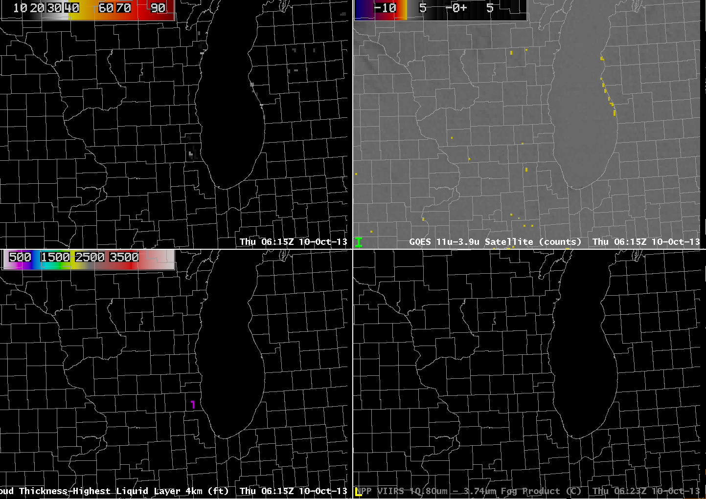
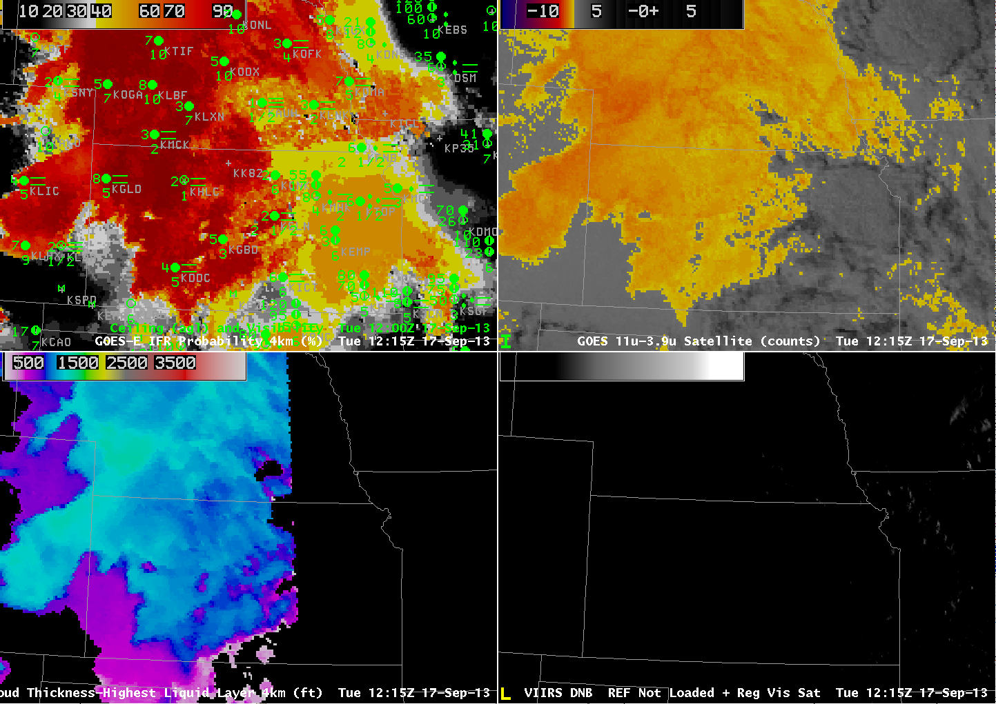
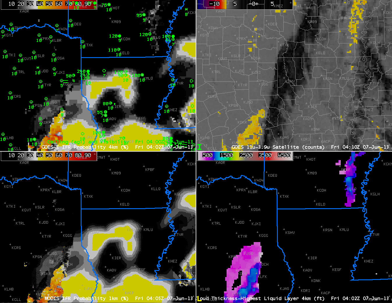
GOES-13-based GOES-R IFR Probabilities (Upper Left), GOES-13 Brightness Temperature Difference Product (10.7 µm – 3.9 µm) (Upper Right), GOES-13-based GOES-R Cloud Thickness (Lower Left), Suomi/NPP Brightness Temperature Difference (Lower Right), all near 0615 UTC on 10 October (click image to enlarge)
The GOES-R IFR Probability product gave useful advance warning to the development of fog near Lake Michigan’s eastern shore overnight. The image above, from 0615 UTC, shows a flat brightness temperature difference field over the lakeshore counties in Wisconsin and Illinois (values are from -7.1 to -7.3); there are two regions of high values in the IFR Probability field, however: Near Manitowoc WI (values up to 29%) and over southeast WI and northeast IL (values near 20%). So by 0615 UTC on 10 October, IFR Probabilities are suggestive of a nascent fog development.
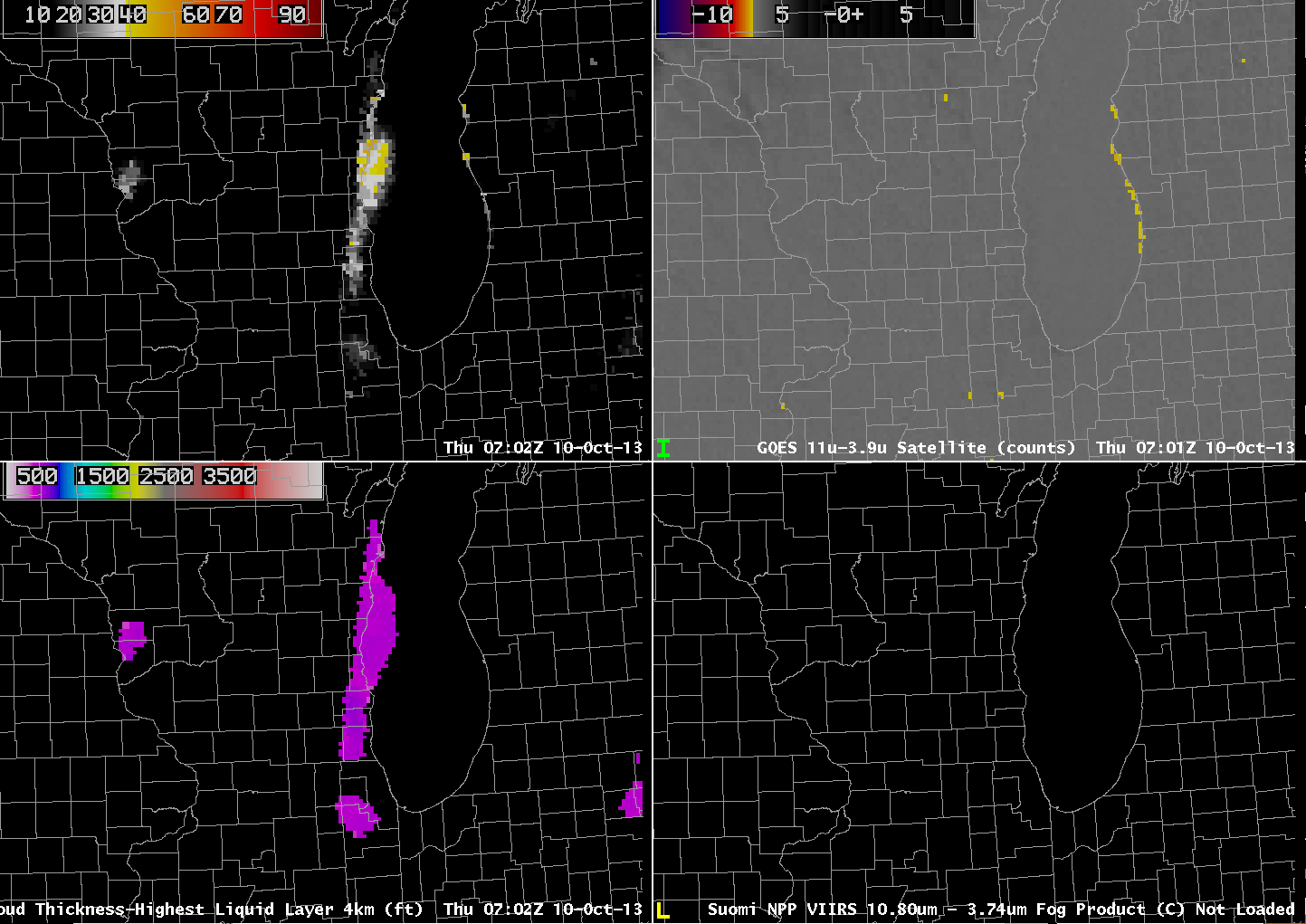
As above, but for 0702 UTC on 10 October (click image to enlarge)
Forty-five minutes later, at 0702 UTC (above), IFR Probabilities have increased dramatically in eastern WI even as the brightness temperature difference field remains flat. Thus, the Rapid Refresh Data is accurately capturing the development of low-level saturation in the atmosphere, and that is influencing the IFR probability field. In addition, the GOES-R Cloud Thickness field is suggesting that the cloud bank is 500-600 feet thick. The strip of enhanced brightness temperature difference paralleling the Lake Michigan shore in lower Michigan is an artifact of the co-registration error between the 10.7 µm and 3.9 µm band detectors on GOES-13. Between 0656 UTC and 0734 UTC, visibility at Manitowoc, WI (KMTW), dropped from 5 to 3/4 statute miles. The visibility at Burlington WI (KBUU) dropped from 4 to 1 statute miles between 0600 and 0700 UTC, and Waukegan, IL (KUGN) reported a visibility of 1/4 mile at 0552 UTC and 0652 UTC.
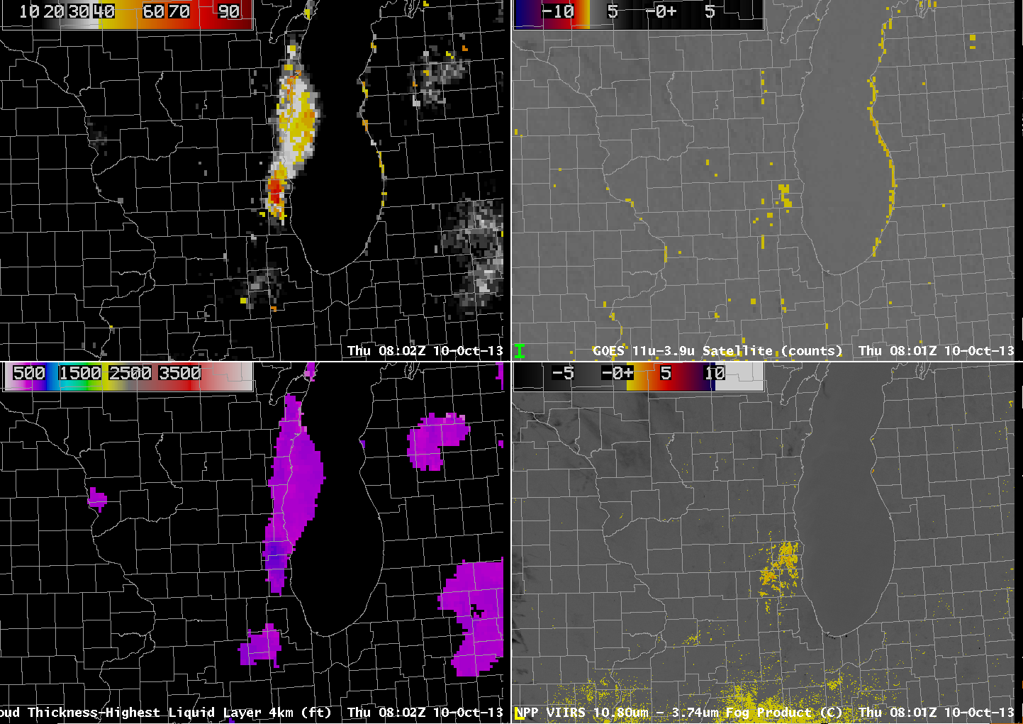
As above, but for 0802 UTC on 10 October (click image to enlarge)
At 0802 UTC, the GOES-East brightness temperature difference field shows greater differences over the region of SE Wisconsin where the fog is developing. Accordingly, the IFR probability increases past 80% IFR Probabilities are near 70% in Manitowoc County (and Manitowoc reported 1/2-mile visibility at 0834 UTC). Compare the GOES-East and Suomi/NPP Brightness Temperature Difference Fields; note the lack of a signal in the Suomi/NPP field along the western shore of Lake Michigan, confirming the co-registration error present in GOES-13.

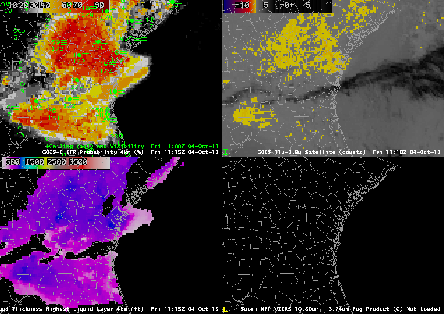
As above, but for 1145 UTC on 10 October (click image to enlarge)
The last pre-sunrise image, 1145 UTC, shows a definite signal of fog/low stratus in both the IFR Probability field and in the Brightness Temperature Difference field. However, the early detection in the IFR Probability field gives a nice head’s up to the forecaster. Note also in this image how the strong signal in the brightness temperature difference field that arises because of the co-registration error can contaminate the IFR Probability field. The Cloud Thickness in this field has been related to dissipation time, as shown in this chart. The maximum thickness of 1000 feet predicts a dissipation time around 1500 UTC. The 1445 and 1515 UTC GOES-13 visible images are shown below.
GOES-13 Visible Imagery at 1445 UTC and 1515 UTC on 10 October (click image to enlarge)
")