Author Archives: Scott Lindstrom

Advection Fog and Multiple Cloud Layers

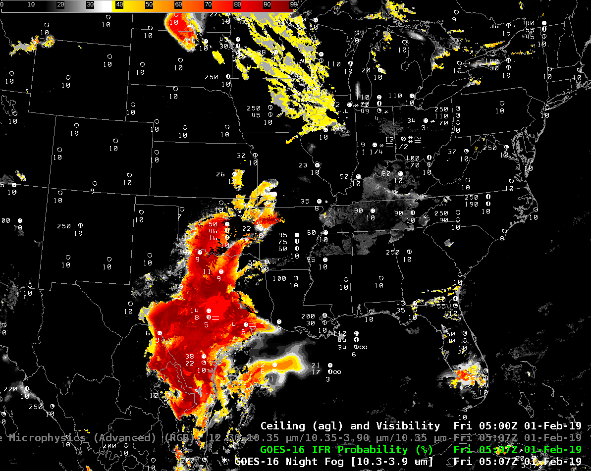
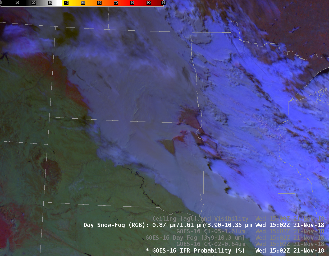
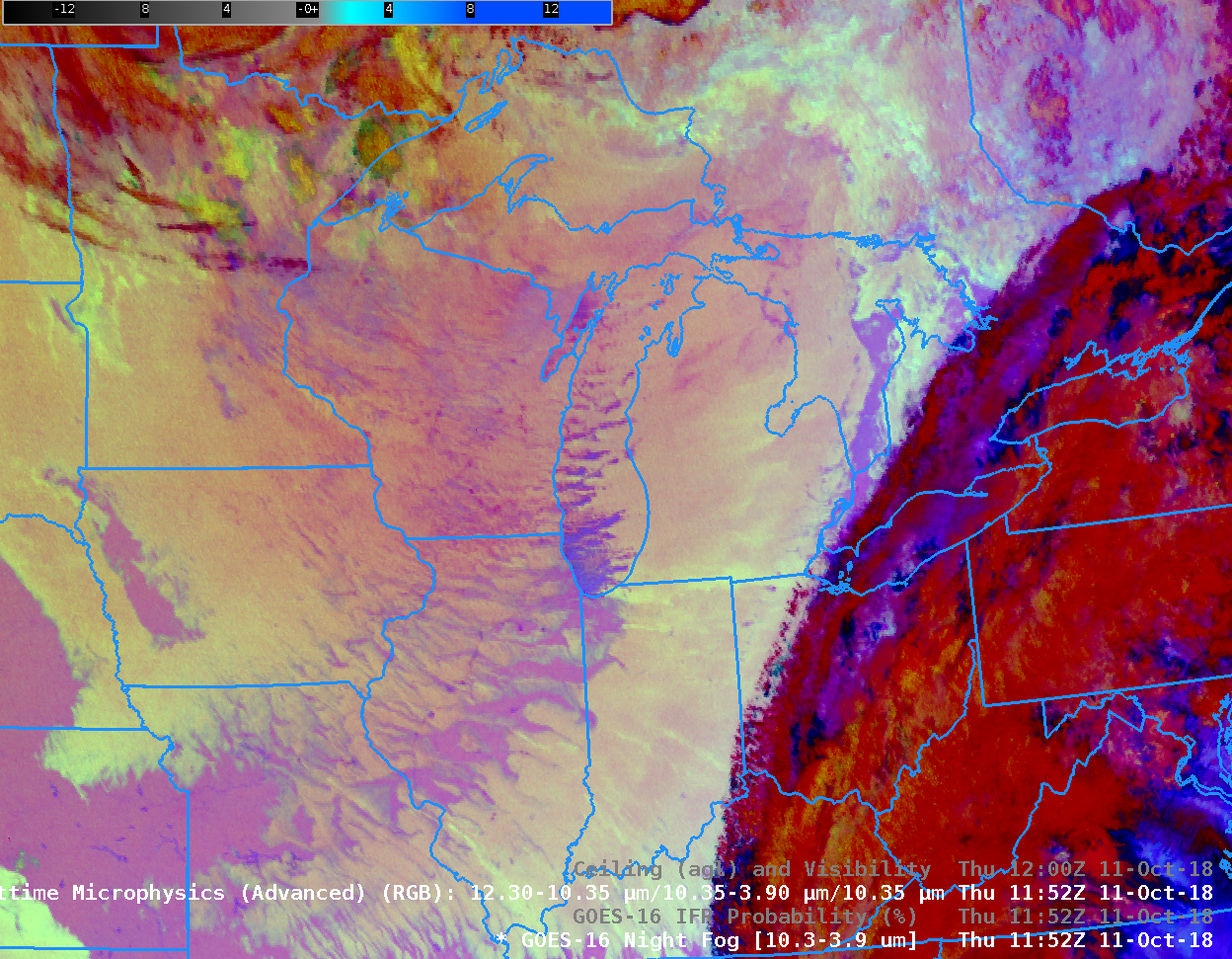
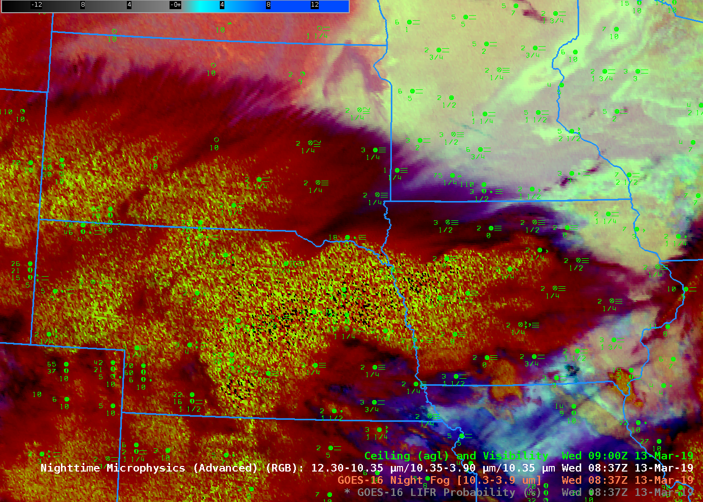
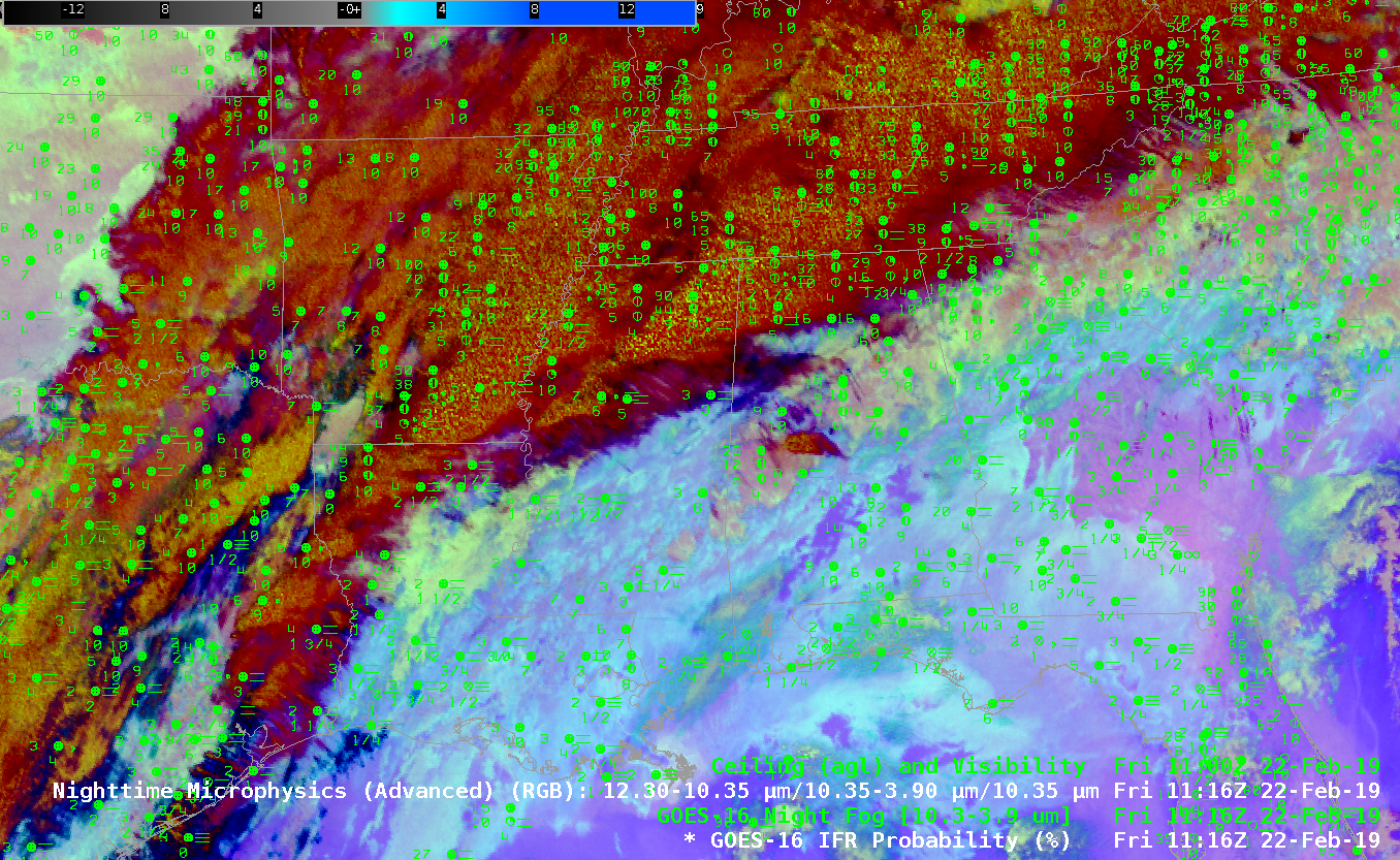
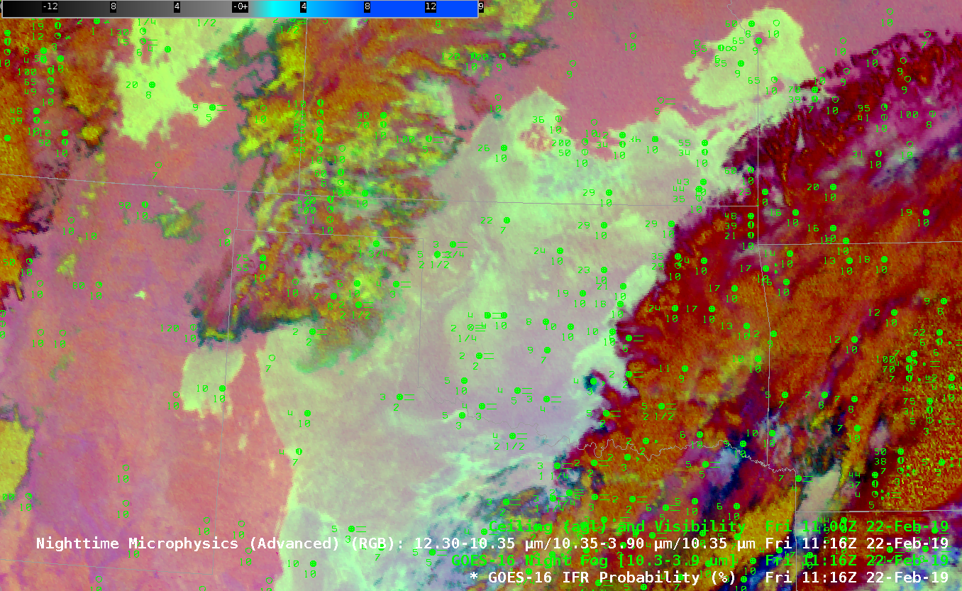
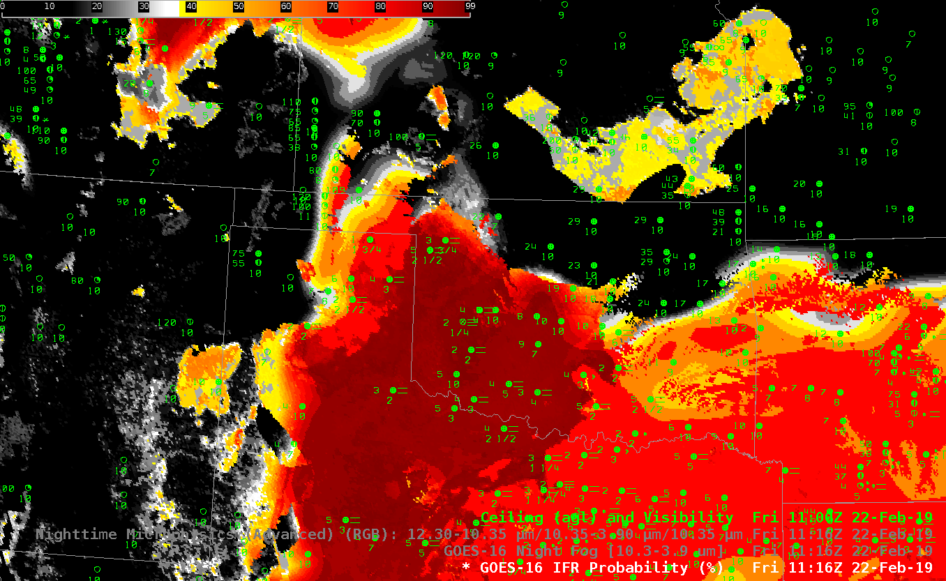
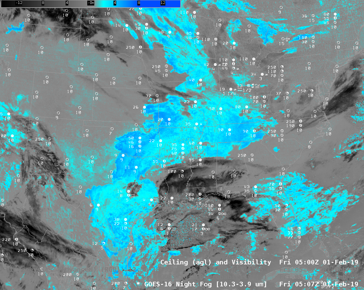
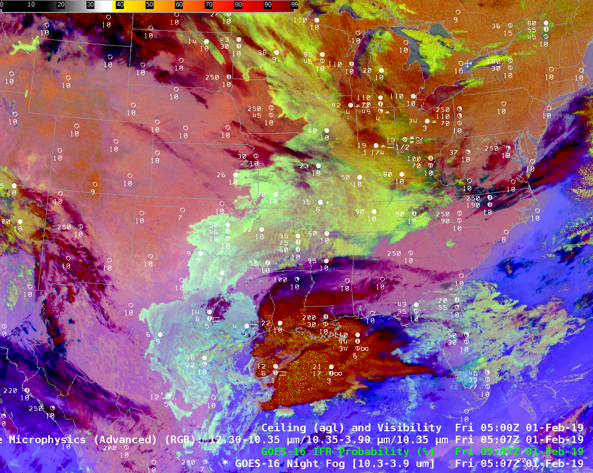
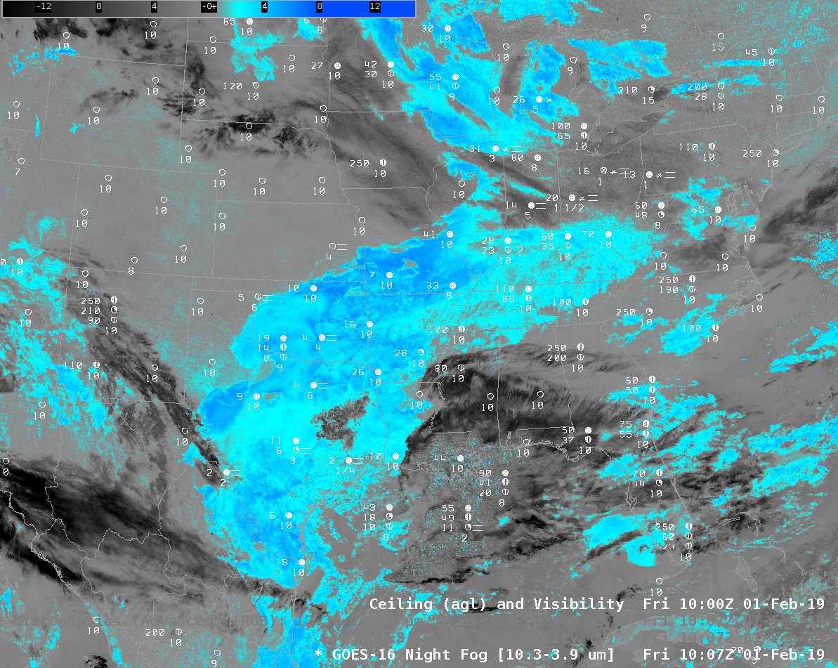
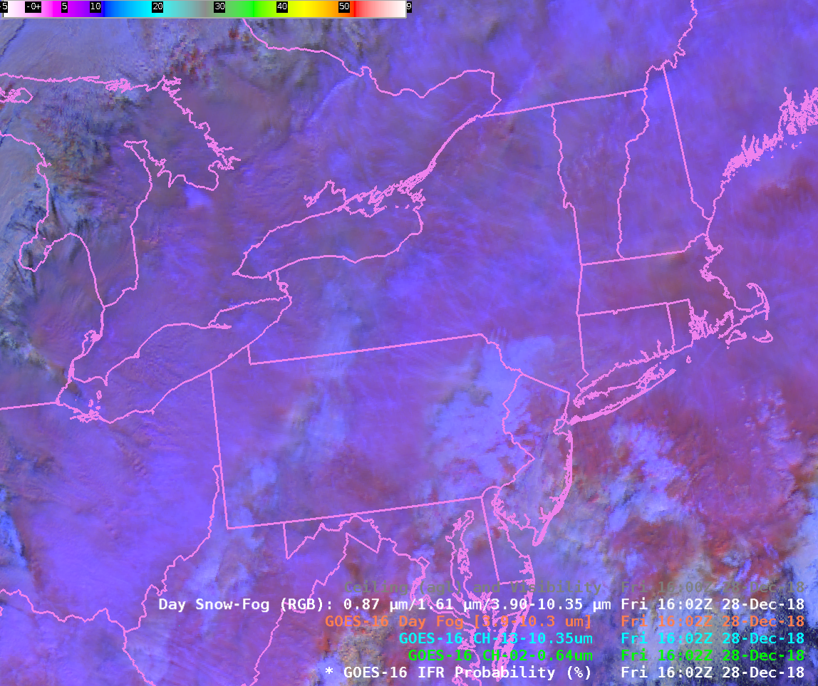
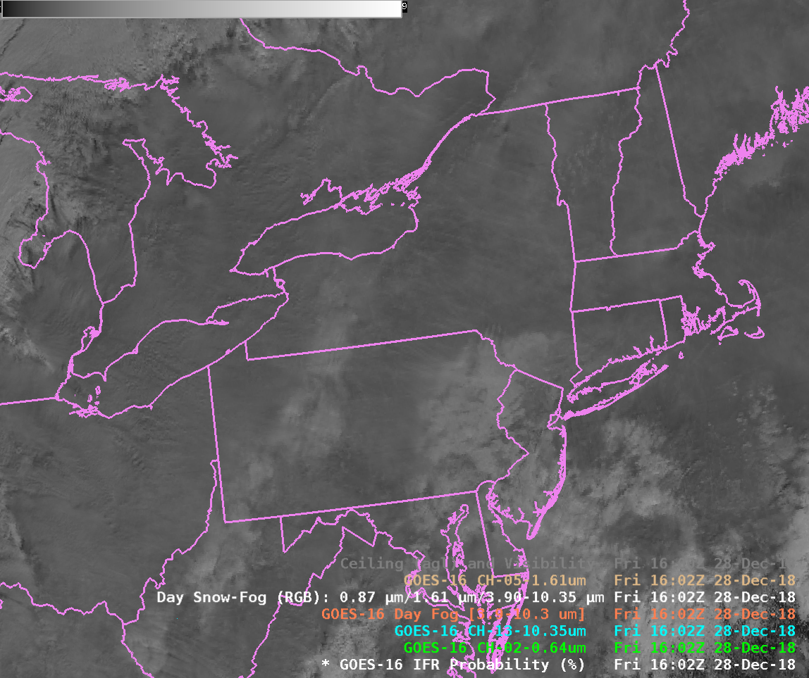
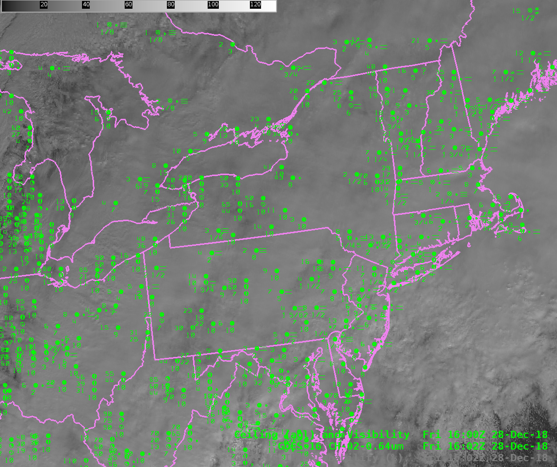
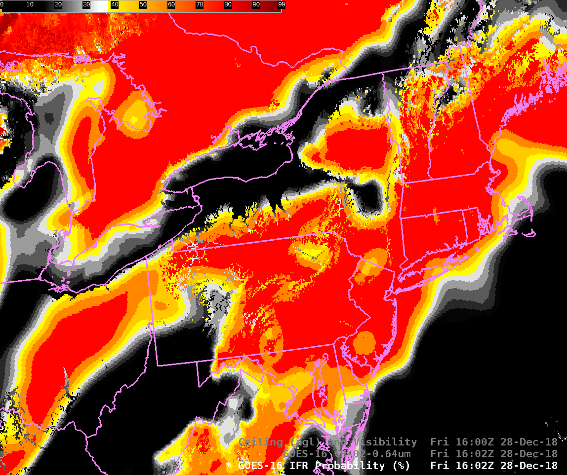
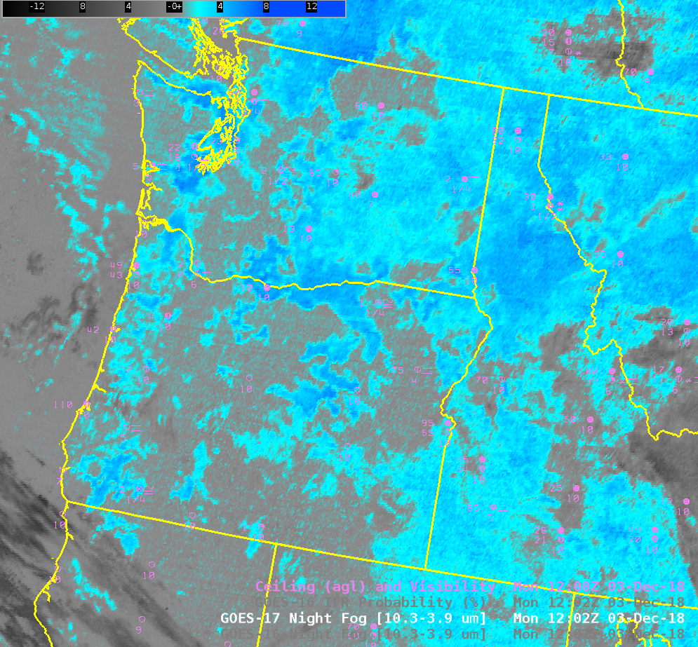
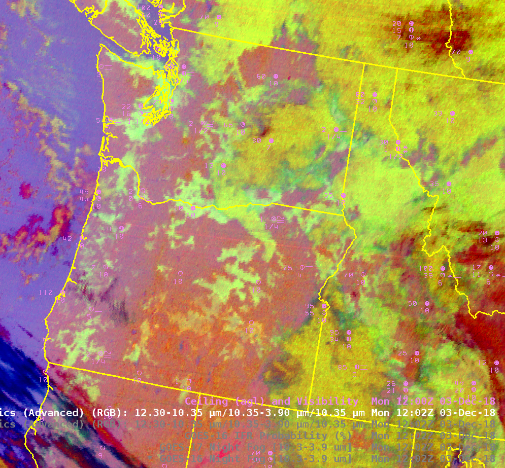
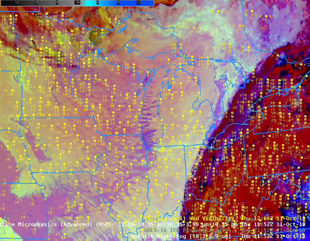
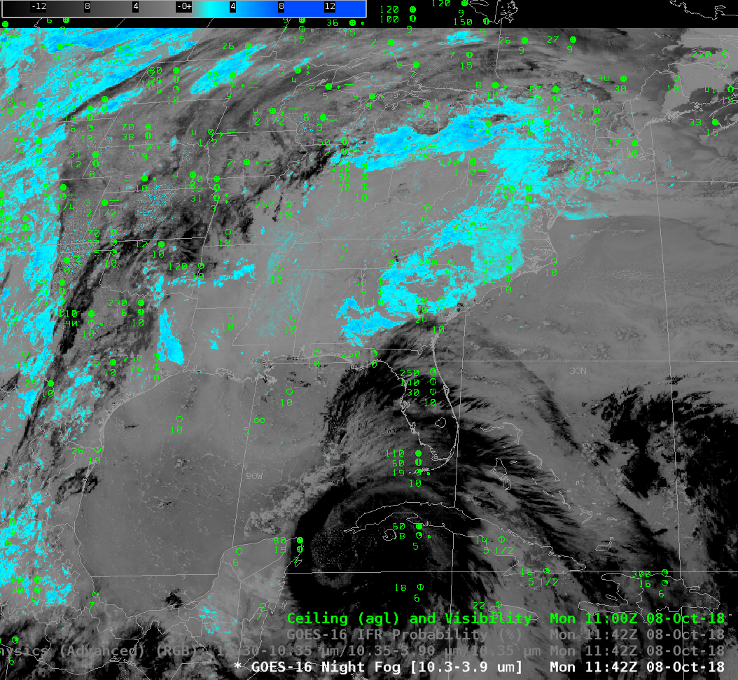
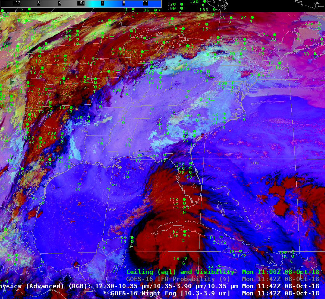
GOES-16 Night Fog Brightness Temperature Difference (10.3 µm – 3.9 µm), Low IFR Probability and Advanced Nighttime Microphysics RGB at 0837 UTC on 13 March 2019 (Click to enlarge)

An intense early Spring storm produced blizzard conditions over the western Great Plains on 13 March 2019 (See this blog post for example). The southerly flow in advance of the storm moved moist air over a dense snowpack over the upper Midwest, resulting in dense Advection Fog. The animation above cycles between the Night Fog Brightness Temperature Difference (10.3 µm – 3.9 µm), the Advanced Nighttime Microphysics RGB that uses the Night Fog Brightness Temperature Difference as the ‘green’ and GOES-16 Low IFR Probabilities.

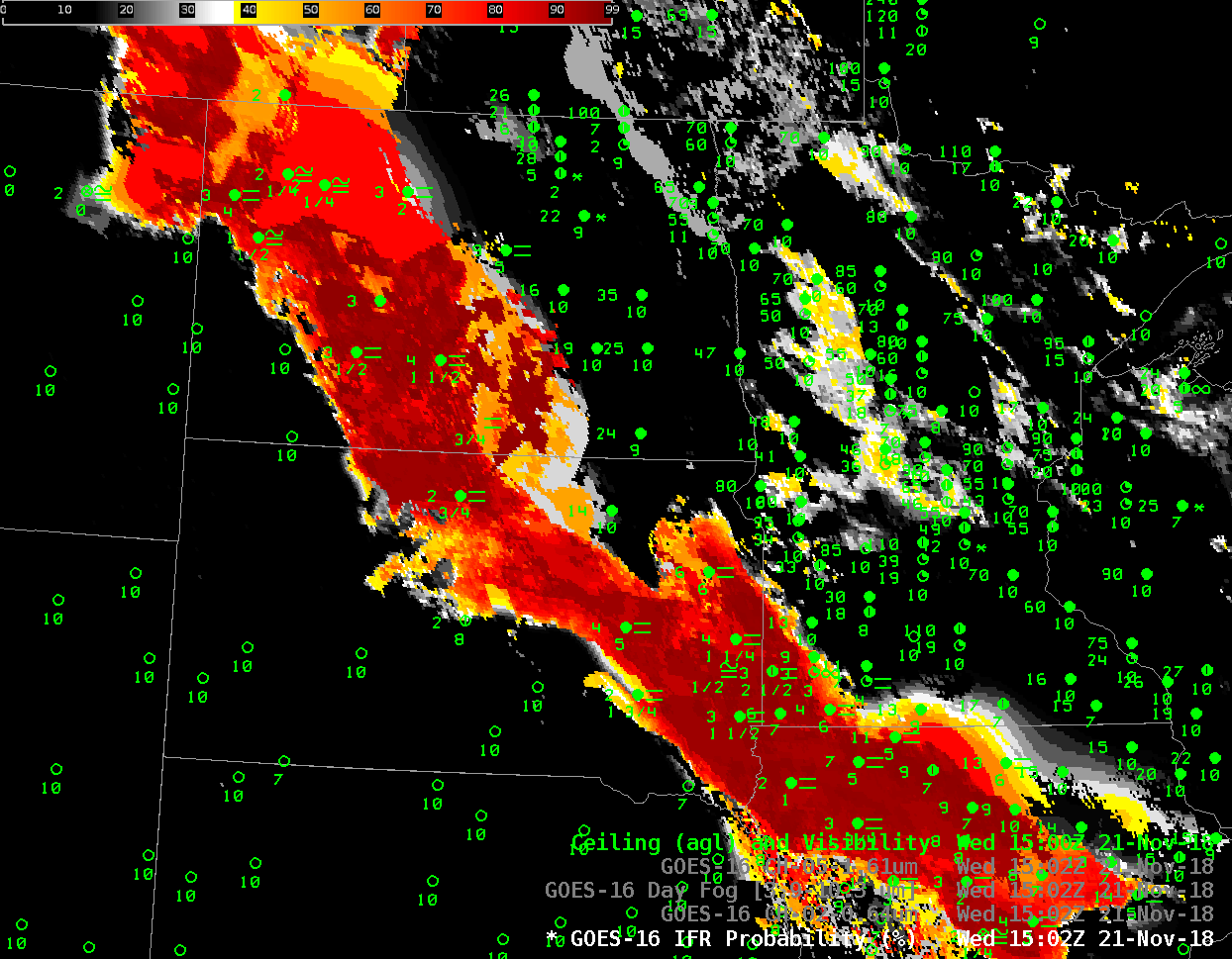
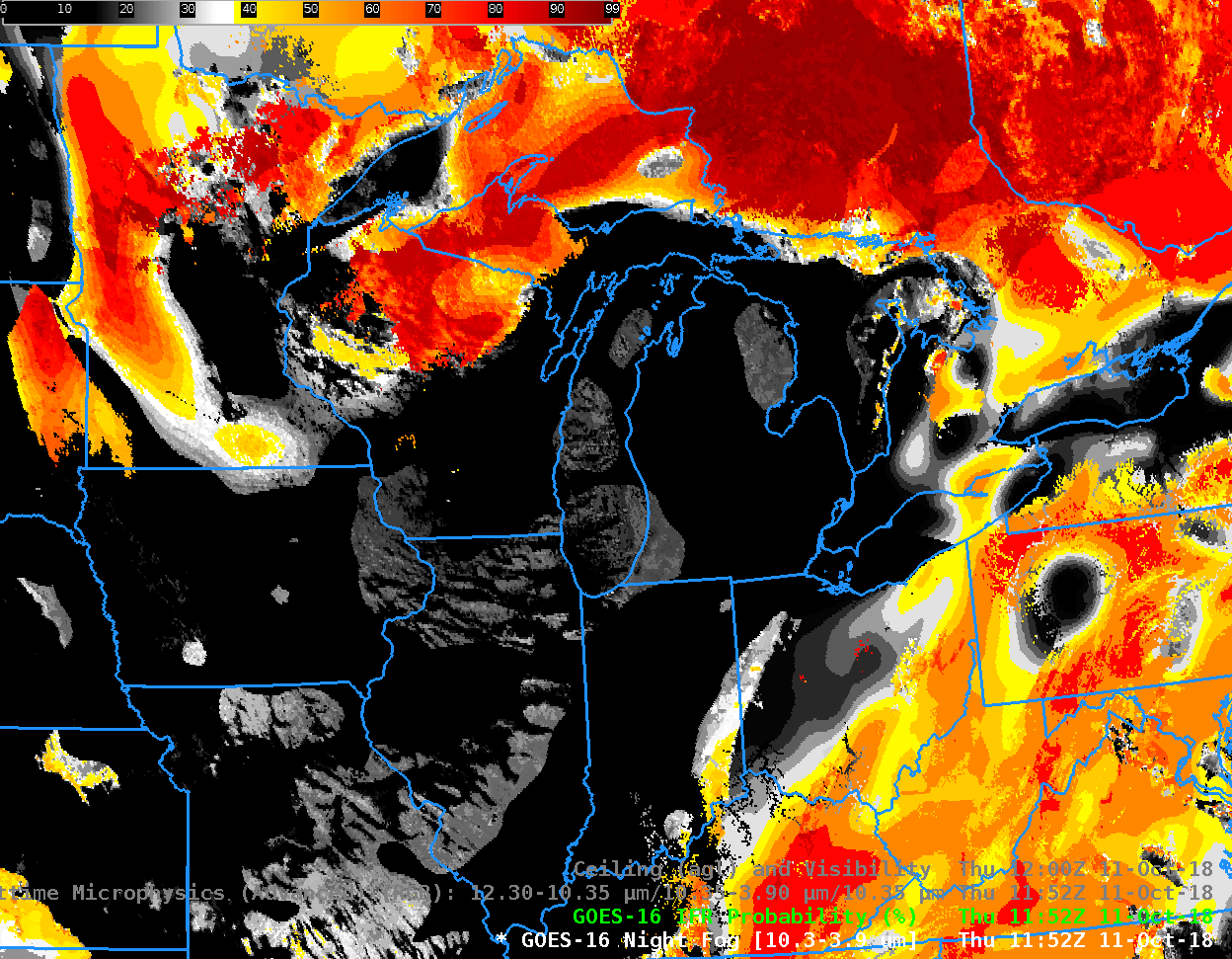
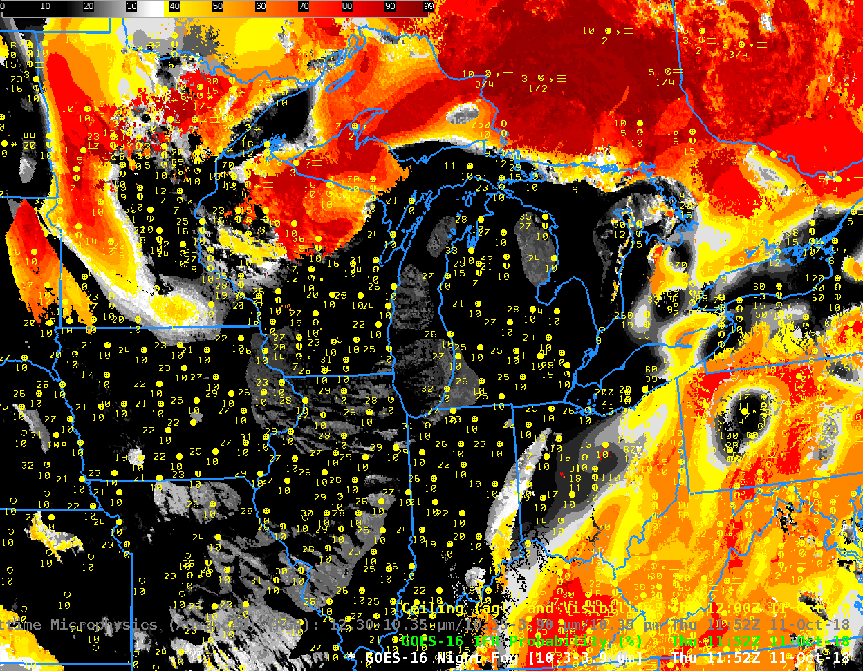
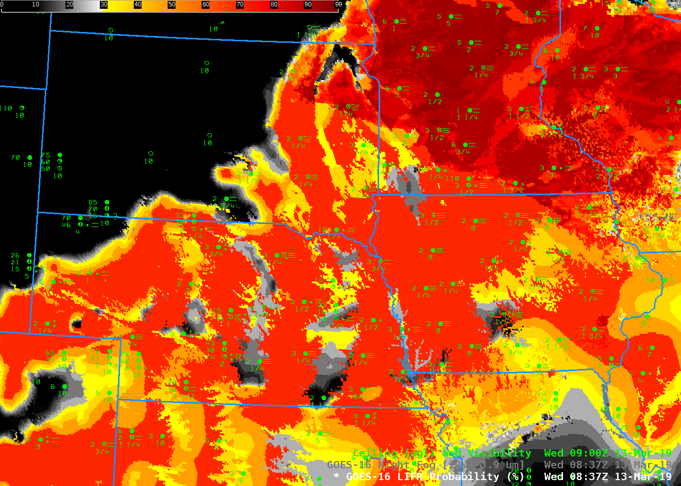
At 0837 UTC, high clouds had not yet covered all of the upper Midwest, and the satellite still viewed stratus clouds over Wisconsin and Minnesota (bright cyan in the Night Fog Brightness Temperature difference enhancement). Note the difference in the Low IFR Probability field in regions where high clouds are present (Iowa and states to the south and west) and where they are not. Low IFR Probability has a pixelated look over Wisconsin because modest satellite pixel-level variability is included in the IFR probability field. Over Iowa, in contrast, satellite data gives no information about reductions to visibility under the thick cloud cover; low-level data from the Rapid Refresh model drives the Low IFR Probability field there. Probabilities are high in regions where observations suggest IFR/Low IFR conditions are present. This suggest the Rapid Refresh is simulating the evolution of the atmosphere well over the Plains.

The Advanced Nighttime Microphysics RGB can detect low clouds — but only when high clouds are not in the way. For this case, the RGB signal over Wisconsin is consistent with stratus and fog, but over Iowa the signal is consistent with cirrus that is occurring there. Surface restrictions in visibility and lowered ceilings are similar in the two states, and the IFR Probability field has similar values in the two states.

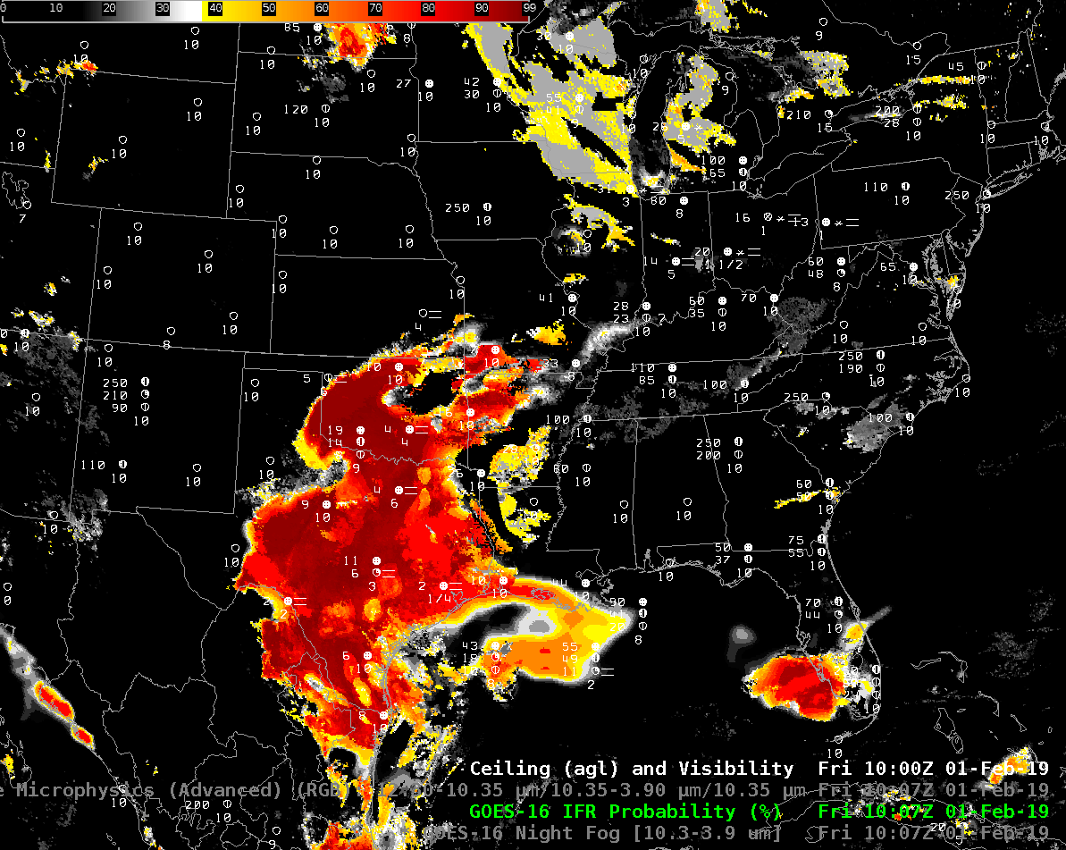
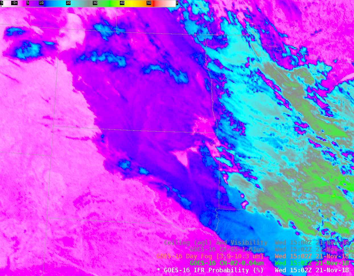
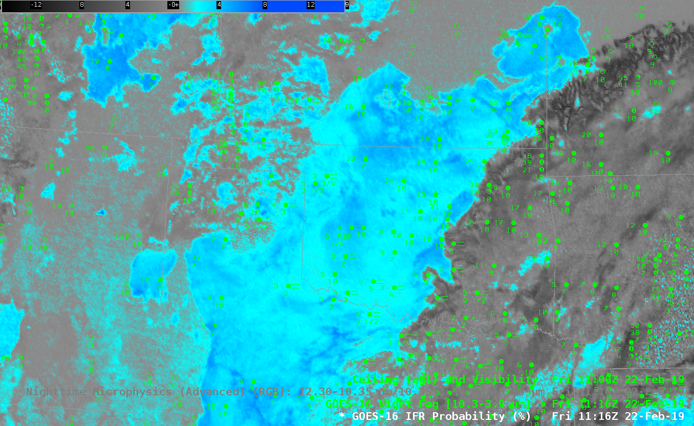
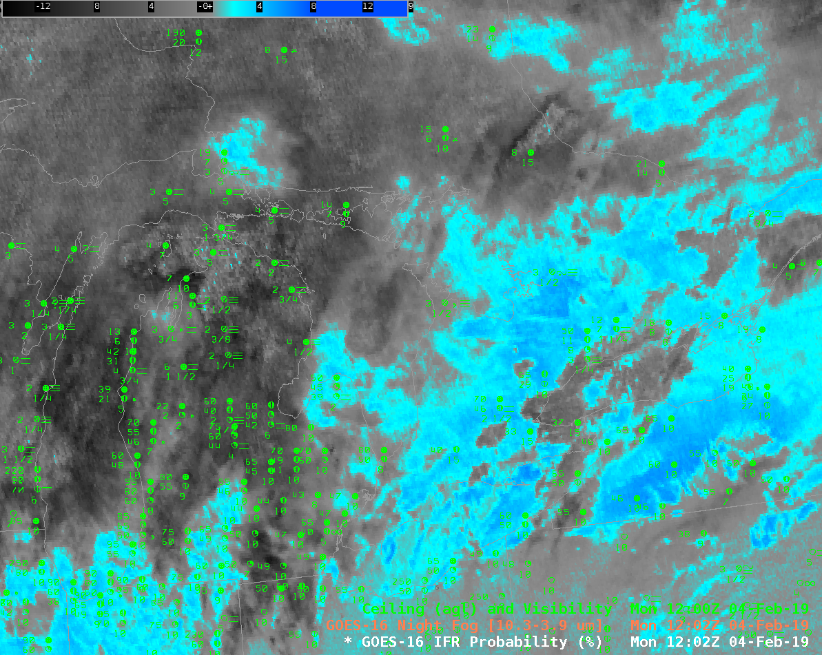
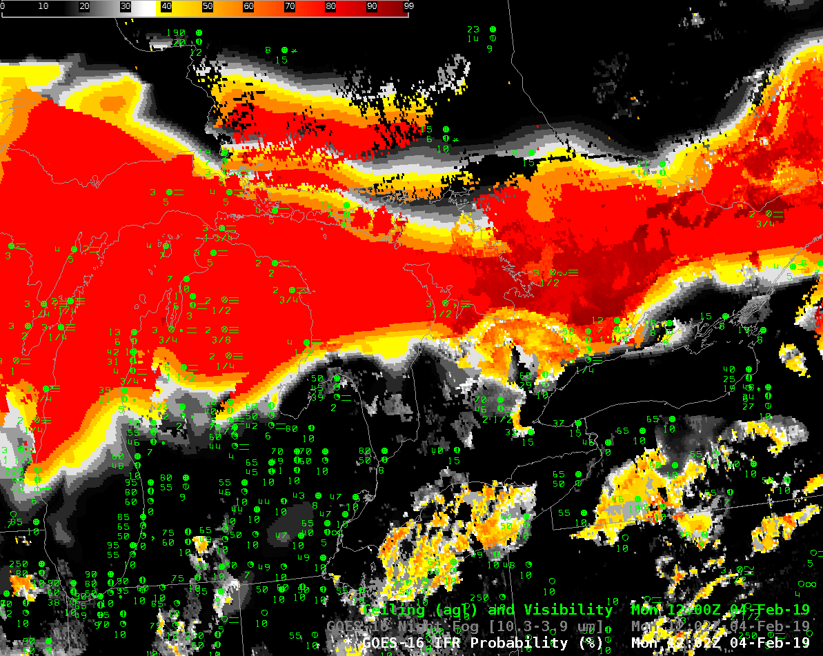
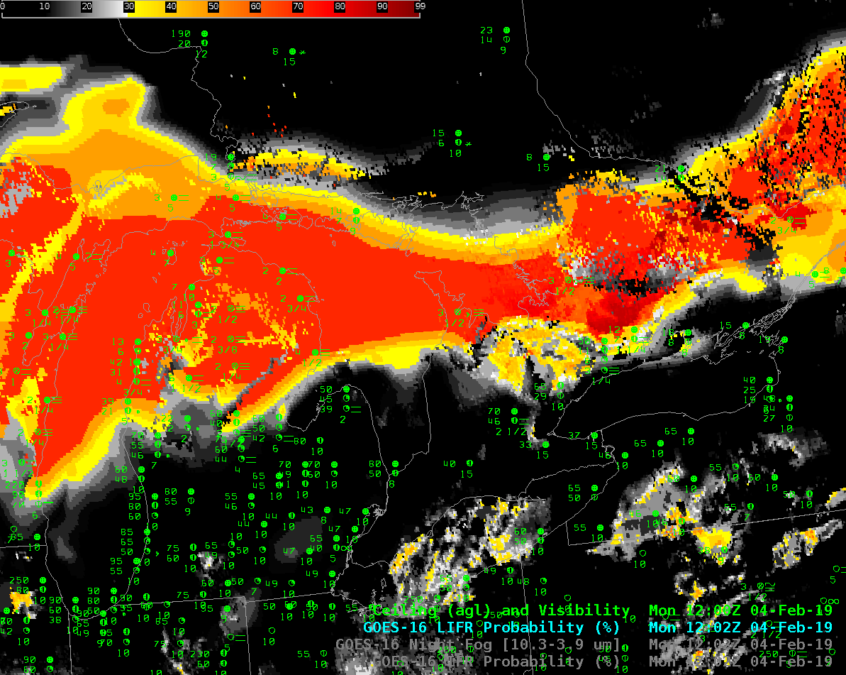
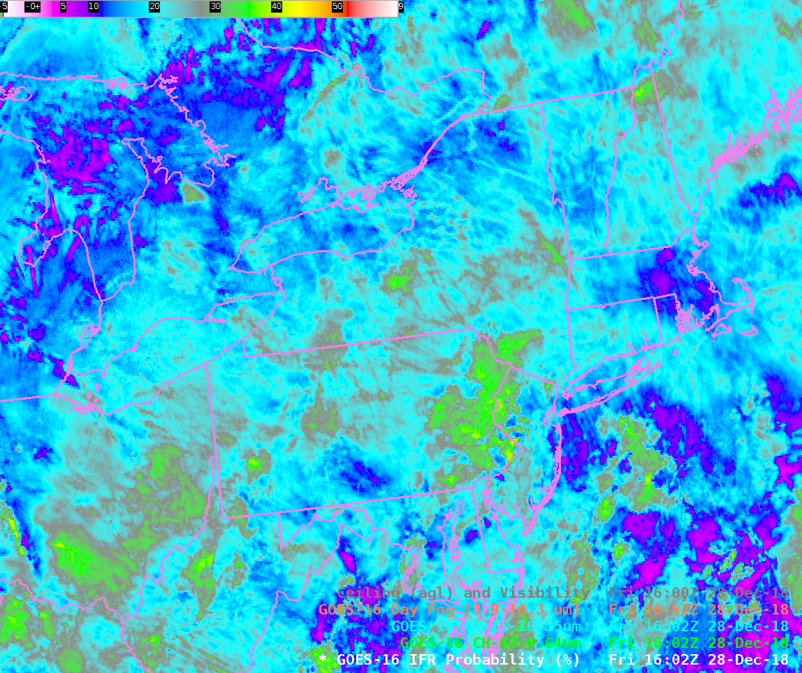
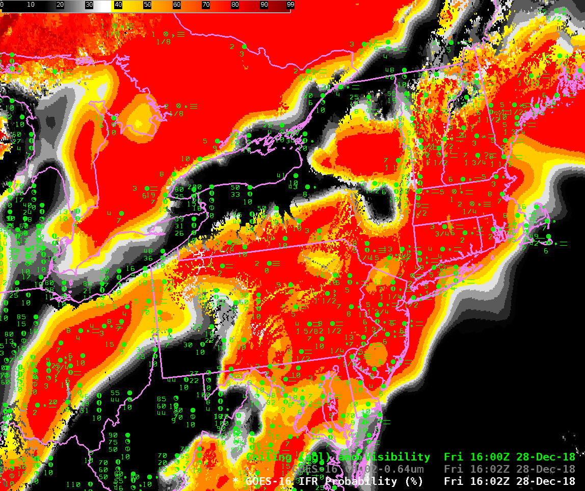
By 1502 UTC on 13 March (below), high clouds had overspread the entire Midwest; Low IFR Probability relies almost entirely on Rapid Refresh Model estimates of low-level saturation.  That is why the field over northern Minnesota and northern Wisconsin is flat.  Some holes in the high clouds are suggested by the pixelated look of the field in Iowa and southern Wisconsin.

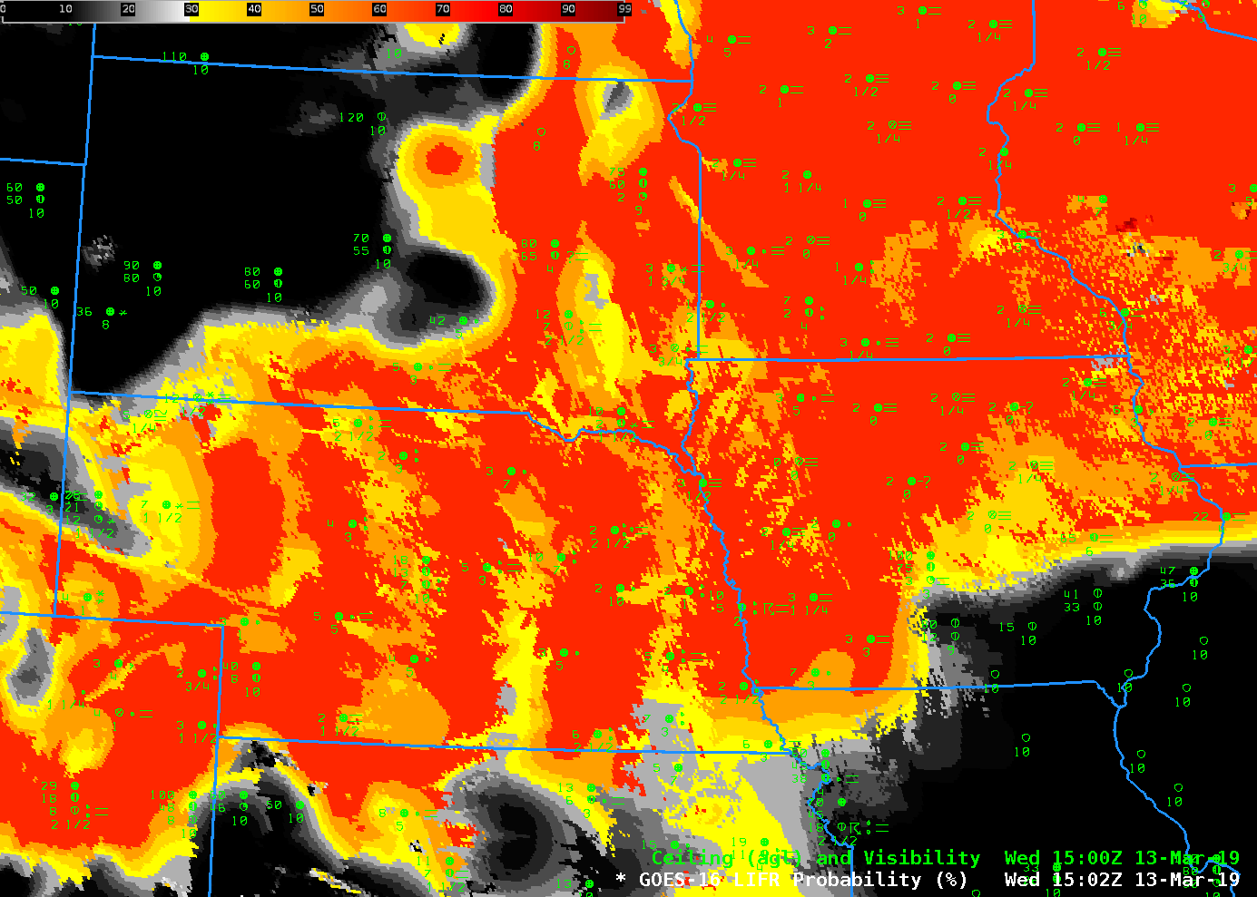
GOES-16 Low IFR Probability, 1502 UTC on 13 March 2019 (Click to enlarge)

Cloud Layers and Detection of IFR Conditions

GOES-16 Night Fog Brightness Temperature Difference (10.3 µm – 3.9 µm), Nighttime Microphysics RGB and GOES-16 IFR Probability at 1116 UTC on 22 February 2019; Surface observations of ceilings and visibilities at 1100 UTC are also plotted (Click to enlarge).

A strong storm embedded within a subtropical jet stream over the southern United States was associated with widespread fog on the morning of 22 February 2019. This screen-capture from this site shows Dense Fog Advisories over much of Georgia, and over regions near Dallas. Which products allowed an accurate depiction of the low ceilings and reduced visibilities?

The toggle above cycles between the Night Fog Brightness Temperature Difference (10.3 µm – 3.9 µm), which product identifies low clouds (cyan blue in the default AWIPS enhancement shown) because of differences in emissivity at 3.9 µm and 10.3 µm from small water droplets that make up stratus clouds, the Nighttime Microphysics RGB, which RGB uses the Night Fog Brightness Temperature Difference as it green component, and the GOES-16 IFR Probability product.  IFR conditions are defined as surface visibilities between 1 and 3 miles, and ceiling heights between 500 and 1000 feet above ground level.  The plotted observations help define where that is occurring.  Multiple cloud layers from Arkansas east-northeastward make a satellite-only detection of IFR conditions challenging.  IFR Probability gives useful information below cloud decks because model-based saturation information from the Rapid Refresh Model fill in regions below multiple cloud decks where satellite information about low clouds is unavailable.

The toggle below shows the same three satellite-based fields (Night Fog Brightness Temperature Difference, Nighttime Microphysics RGB and IFR Probability)  at the same time, but centered over Oklahoma.  In this case, the Rapid Refresh Data are used to screen out a region of elevated stratus over northeast Oklahoma. Note that these is little in the Night Fog Brightness Temperature Difference field to distinguish between the IFR and non-IFR locations.

GOES-16 Night Fog Brightness Temperature Difference (10.3 µm – 3.9 µm), Nighttime Microphysics RGB and GOES-16 IFR Probability at 1116 UTC on 22 February 2019; Surface observations of ceilings and visibilities at 1100 UTC are also plotted (Click to enlarge).

GOES-R IFR Probability over the southeast United States in this case is identifying regions of IFR conditions underneath multiple cloud decks (and also where only the low clouds are present) by incorporating low-level saturation information from the Rapid Refresh model. Over Oklahoma, non-IFR conditions under an elevated stratus deck are identified (and screened out in IFR Probability fields) by the lack of low-level saturation information in the Rapid Refresh.

Advection Fog in Warm Air Advection Regimes

‘Night Fog’ Brightness Temperature Difference field (10.3 μm – 3.9 μm) and GOES-R IFR Probability at 1202 UTC on 4 February 2019 (Click to enlarge)

Advection Fog during thaws, when very cold surfaces are overrun by air with dewpoints above freezing, can be very dense, and very difficult to detect via satellite; typically advection fog accompanies extratropical cyclones and their accompanying multiple cloud layers. The toggle above compares the ‘Night Fog’ Brightness Temperature Difference field (10.3 μm – 3.9 μm), historically used to detect low stratus because of radiation emissivity differences of clouds made up of water droplets at those two wavelengths, and GOES-R IFR Probability which fuses information from the satellite — not particularly useful in this case as far as low-level visibility is concerned — with information about low-level saturation from the Rapid Refresh Model. GOES-R IFR Probability gives a much more accurate depiction of exactly where the reduced visibilities and lowered ceilings are present, a vital piece of information for aviation (for example).

In addition, Low IFR Probability suggests where the lowest ceilings and greatest visibility reductions occur. The toggle below compares IFR Probability and Low IFR Probability at 1202 UTC (Here’s the toggle at 1642 UTC).  As expected, the region of Highest Low IFR Probability is contained within the region of highest IFR probability;  values of Low IFR Probability are somewhat smaller than those for IFR Probability (the same colorscale is used for both products).

GOES-R IFR Probability and Low IFR Probability at 1202 UTC on 4 February 2019 (Click to enlarge)

Fog over the central United States

Night Fog Brightness Temperature Difference (10.3 µm – 3.9 µm) and Nighttime Microphysics RGB at 0507 UTC on 1 February 2019, and surface observations of ceilings and visibilities (Click to enlarge)

The toggle above displays the Night Fog Brightness Temperature Difference field (10.3 µm – 3.9 µm) and the Night Time Microphysics Red/Green/Blue (RGB) Product that uses the Night Fog Brightness Temprature Difference field as its green value. In the color enhancements above, cyan in the Night Fog Brightness Temperature Difference denotes positive values that occur because stratus clouds — that is, clouds that are made up of water droplets — do not emit 3.9 µm radiation as a blackbody. Consequently, the computation of brightness temperature (which assumes blackbody emission) results in a 3.9 µm brightness temperature that is cooler than at 10.3 µm (clouds are emitting 10.3 µm radiation very nearly like a blackbody).  Low clouds in the RGB that may or may not support IFR conditions range in color from light cyan (over Texas and Florida) to more orange and yellow (yellow over the Great Lakes were exceptionally cold air is in place).

The fields above are overpredicting where fog/low ceilings might be occurring because cloud top measurements from the Brightness Temperature Difference do not always give reliable guidance on cloud base.

By merging satellite information about clouds and cloud type with Rapid Refresh model information at about low-level saturation, GOES-R IFR Probability fields screen out regions where IFR conditions are unlikely;  the map suggests low ceilings and fog are most likely over Texas and Oklahoma.  The zoomed in image, below shows that IFR conditions are indeed occurring in this region.  Other regions with a strong signal in the Brightness Temperature Difference field — Tennessee, for example — show low IFR Probability and surface observations that do not show IFR conditions.

GOES-R IFR Probability field, 0507 UTC on 1 February, along with surface reports of ceilings and visibility (Click to enlarge)

GOES-R IFR Probability field, 0507 UTC on 1 February, along with surface reports of ceilings and visibility zoomed in over the southern Plains (Click to enlarge)

Night Fog Brightness Temperature Difference (10.3 µm – 3.9 µm) and Nighttime Microphysics RGB at 1007 UTC on 1 February 2019, and surface observations of ceilings and visibilities (Click to enlarge)

The same relationships occur at 1007 UTC; the Night Fog Brightness Temperature Difference and Nighttime Microphysics RGB overpredict the regions of low clouds/fog; IFR Probability’s use of Rapid Refresh Data allows it to screen out regions where fog is not present, but stratus clouds are, and also add in regions where cirrus clouds prevent the detection of low clouds, but Rapid Refresh data suggests low-level saturation is present (such as over the Gulf of Mexico south of Louisiana).

The IFR Probability field is accurately outlining the region of IFR conditions.

GOES-R IFR Probability field, 1007 UTC on 1 February, along with surface reports of ceilings and visibility (Click to enlarge)

GOES-R IFR Probability field, 1007 UTC on 1 February, along with surface reports of ceilings and visibility zoomed in over the southern Plains (Click to enlarge)

Fog over the Northeast: Where is it?

GOES-16 ABI Band 02 (0.64 µm), Band 13 (10.3 µm), Day Fog Brightness Temperature (3.9 µm – 10.3 µm), Day Snow Fog RGB and Band 5 (1.61 µm) at 1602 UTC on 28 December 2018 (Click to enlarge)

The animation above cycles through the GOES-16 Visible Imagery (Band 2, 0.64 µm), Band 13 (Clean Window Infrared, 10.3 µm), the Day Fog Brightness Temperature Difference (3.9 µm – 10.3 µm), the Day Snow Fog Red Green Blue (RGB) Composite and the Snow/Ice near-Infrared channel (Band 5, 1.61 µm) that is the green component of the Day Snow Fog RGB. (That’s very apparent in this toggle between the Day Snow Fog RGB and the 1.61 µm) Do any of these products give you a good idea of where IFR conditions (Low ceilings and reduced visibilities) are occurring?

Consider the toggle of visible imagery below, with and without surface observations of ceilings and visibility. It is a difficult prospect to relate the top-of-cloud reflectance (which is what the visible imagery gives you!) to the ceilings beneath the cloud.

GOES-16 ABI Band 02 (0.64 µm) with an without surface observations of ceilings and visibility at 1602 UTC on 28 December 2018 (Click to enlarge)

GOES-16 IFR Probability fields blend satellite observations of cloud with Rapid Refresh model data that predicts saturation near the surface. That model data, incorporated into a statistical prediction of IFR conditions, allows the field to outline the regions where low ceilings and reduced visibilities occur, as shown in the toggle below with and without observations. (Click here to see the Visible and IFR Probability fields toggled). The inclusion of near-surface saturation values extracted from the Rapid Refresh model allows the IFR Probability field to discriminate between low ceilings/fog — as over central Pennsylvania, Massachusetts and central Ohio (among other places) — and mid-level stratus — as over southwestern Pennsyvlania and surrounding Lakes Erie and Ontario (among other places).

GOES-16 IFR Probability with surface observations of ceilings/visibilities at 1602 UTC on 28 December 2018 (Click to enlarge)

Fog over the Pacific Northwest: Where is it?

GOES-17 imagery in this blog post is made from GOES-17 Data that are preliminary and non-operational!

Night Time Fog Brightness Temperature Difference (10.3 µm – 3.9 µm) from GOES-16 and (preliminary, non-operational) GOES-17, 1202 UTC on 3 December 2018 (Click to enlarge)

The toggle above shows GOES-16 and GOES-17 Night Fog Brightness Temperature difference fields over the Pacific Northwest shortly after 1200 UTC on 3 December 2018.  The Pacific NW is a lot farther from the sub-satellite point (nadir) of GOES-16 (75.2 West Longitude) than from the sub-satellite point (nadir) of GOES-17 (at 137.2 W Longitude).  Thus, the GOES-16 view is has inferior spatial resolution.  There are also different parallax shifts for clouds between the two views.  The scene includes plenty of stratus, based on the observations, and isolated pockets of IFR conditions:  Spokane WA, Stampede Pass, WA, Pendleton OR, Medford OR, Salem OR.  It’s difficult to tell at a glance from the Brightness Temperature Difference field where the lowest ceilings and poorest visibilities are — because the satellite sees the top of the cloud, and it’s difficult to infer cloud base properties from infrared imagery of the cloud top.

The Advanced Nighttime Microphysics RGB can also be used to detect low ceilings, because its green component is the Night Fog Brightness Temperature Difference as shown above.  The toggle below compares the GOES-16 and GOES-17 RGBs.  Again, it is difficult to pinpoint at a glance where the IFR conditions are occurring in this product.

There are subtle differences in the colors of the RGB from the two satellites.  These are related to the distance from the sub-satellite point.  Limb cooling will cause the brightness temperatures from the GOES-16 Clean Window to be slightly cooler than the GOES-17 values, and that will affect the color:  The Clean Window is the Blue component of the RGB.  In addition, the Split Window Difference values will be slightly different because of the different amounts of limb cooling in 12.3 µm and 10.3 µm brightness temperatures.  GOES-17 data also includes striping that is being addressed with ongoing calibration work with the satellite.

Advanced Nighttime Microphysics RGB from GOES-16 and GOES-17 at 1202 UTC on 3 December 2018 (Click to enlarge)

The toggle below shows, (from GOES-16 data) the 10.3 µm – 3.9 µm Brightness Temperature Difference, the Nighttime Microphysics RGB, and the IFR Probability fields at 1202 UTC. IFR Probability fields include information about low-level saturation from the Rapid Refresh model, and that information allows the product to screen out regions of mid-level stratus; thus, the region of IFR conditions is better captured.  There are three main regions:  eastern WA southwestward to Pendleton OR, Seattle southward into Oregon, and the peaks of central Washington.

GOES-16 Night Fog Brightness Temperature Difference (10.3 µm – 3.9 µm), Nighttime Microphysics RGB and IFR Probability, 1202 UTC on 3 December 2018 (Click to enlarge)

Fog over the Dakotas and Minnesota: Where is it?

GOES-16 “Red Visible” Band 2 0.64 µm imagery at 1502 UTC on 21 November 2018 (Click to enlarge)

Consider the GOES-16 Visible (Band 2, 0.64 µm) Image above.  Where is the fog in this image?  Certainly you can tell where clouds exist, and if animated, you could identify snow on the ground (because it wouldn’t move like clouds do).  Alternatively, you could toggle between the visible and the Snow/Ice band (Band 5, 1.61 µm), below;  regions of snow/ice — such as in western North Dakota, or northeastern South Dakota, or Ontario appear bright in the 0.64 µm but dark in the 1.61 µm.

GOES-16 “Red Visible” Band 2 0.64 µm imagery and “Snow/Ice” Band 5 1.61 µm imagery at 1502 UTC on 21 November 2018 (Click to enlarge)

The Day Fog Brightness Temperature Difference product (3.9 µm – 10.3 µm) highlights low clouds. Stratus clouds with water droplets are scatterers of incoming solar radiation. The clouds over Minnesota and Iowa appear to be composed of much smaller water droplets, however, because they are so much warmer — the brightness temperature difference is much larger.  Smaller droplets are better scatterers of incoming solar radiation.  The image below shows the field, also at 1502 UTC on 21 November.  Are there any differences in this field that suggests fog might be present in one location, but not in the other?

GOES-16 Day Fog Brightness Temperature Difference (3.9 µm – 10.3 µm) imagery at 1502 UTC on 21 November 2018 (Click to enlarge)

The Day Snow Fog RGB composite, below, highlights regions of low clouds, snow/ice, and higher clouds.  Snow (and clouds made of ice) are shaded red, low clouds are shades of grey/blue.  Where is the fog?

GOES-16 Day Snow Fog RGB imagery at 1502 UTC on 21 November 2018 (Click to enlarge)

GOES-R IFR Probability Fields are a better predictor of where IFR conditions (that is, reduced visibility and lowered ceilings as might occur with fog) are occurring.  It combines satellite information and low-level informatio0n about saturation (from the Rapid Refresh model).  This fusing of data accentuates a satellite strength (detection of low clouds made up of water droplets — that is, stratus) and the model strength (namely, where are the low-level saturated?)   In the image below, fog and high probabilities of IFR conditions neatly overlap.  This toggle is between the visible, Day Snow-Fog RGB and IFR Probability field.

GOES-16 IFR Probability at 1502 UTC on 21 November 2018 along with surface observations of ceilings and visibility (Click to enlarge)

Fog under multiple cloud layers

GOES-16 Night Fog Brightness Temperature Difference (10.3 µm – 3.9 µm), 1137 – 1452 UTC on 31 October 2018 (Click to animate)

Consider the imagery above: The Night Fog Brightness Temperature Difference (10.3 µm – 3.9 µm) product can be used to highlight regions of low clouds (cloud made up of water droplets) because those water droplets do not emit 3.9 µm radiation as a blackbody (but do emit 10.3 µm radiation nearly as a blackbody), and the conversion of sensed radiance to brightness temperature assumes blackbody emissions. Thus, the 10.3 µm brightness temperature is warmer than at 3.9 µm. In the enhancement used, low stratus clouds are shades of cyan. Is there fog/low stratus along the coast of the Pacific Northwest? How far inland does it penetrate. It is impossible in this case (and many similar cases) to tell from satellite imagery alone because multiple cloud layers associated with a storm moving onshore prevent the satellite from seeing low clouds. The animation shows the Brightness Temperature Difference field along with surface reports of visibility and ceilings.  IFR and near-IFR conditions are widespread, but there is little correlation between their location and the satellite-only signal.

GOES-16 Night Fog Brightness Temperature Difference (10.3 µm – 3.9 µm), 1137 – 1452 UTC on 31 October 2018, along with surface reports of ceilings (AGL) and visibility (Click to animate)

GOES-R IFR Probability fields fuse together satellite information and model data to provide a better estimate of where IFR conditions might be occurring. The animation below, for the same times as above, shows a high likelihood of IFR conditions (as observed) over much of the eastern third of Washington State. The satellite doesn’t give information about the near-surface conditions in this case, but the Rapid Refresh data strongly suggests low-level saturation, so IFR probabilities are high. The field also correctly shows small likelihood of IFR probailities over coastal southern Oregon and northern California. The Rapid Refresh data used have 13-km resolution, however; fog at scales smaller than that may be present — in small valleys for example.

GOES-16 IFR Probabilities, 1137 – 1452 UTC on 31 October 2018 (Click to animate)

IFR Probability can distinguish between stratus and fog

Night Fog Brightness Temperature Difference (10.3 µm – 3.9 µm). 1152 UTC on 11 October (Click to enlarge)

Consider the Night Fog Brightness Temperature Difference product, above. The enhancement is such that blue regions show where 10.3 µm brightness temperatures are warmer than brightness temperatures at 3.9 µm. At night, this occurs because cloud water droplets do not emit as much 3.9 µm radiation as a blackbody; the conversion of the sensed radiation to a brightness temperature assumes blackbody emissions have occurred, however, and as a result, the 3.9 µm brightness temperature is cool. Cloud water droplets do emit as a blackbody at 10.3 µm, so the brightness temperature over cloud water droplets is warmer than the it is at 3.9 µm. Blue, then, signifies stratus clouds in this enhancement. Can you tell where the fog is?  Do you think IFR conditions are occurring wherever the Brightness Temperature Difference field is blue?  How about under the extensive cirrus shield, associated with former Hurricane Michael, that is over the southeastern fifth of the image?

The Advanced NIght time Microphysics RGB for the same time, below, uses as one of its inputs (the ‘green channel’ in the RGB) the Night Fog Brightness Temperature Difference (Click here for a toggle between the two to reinforce that statement).

Night Time Microphysics RGB at 1152 UTC on 11 October (Click to enlarge)

GOES-R IFR Probability fields, below, for the same time are useful because Rapid Refresh model data used in IFR Probability include low-level model estimates of saturation.  If saturation does not exist underneath the cloud deck, then IFR Probabilities are suppressed.  Don’t expect fog, then, underneath the strong signal in the Brightness Temperature Difference field over most of the Midwestern United States!  In addition, the Rapid Refresh Model data defines potential fog under the big cirrus shield over the Appalachians.

GOES-R IFR Probability fields at 1152 UTC on 11 October (Click to enlarge)

Click here for the Advanced Microphyics RGB with observations of ceilings and visibility.  Here are the observations over the Brightness Temperature Difference.  Observations plotted on top of IFR Probability are shown below.

GOES-R IFR Probability fields at 1152 UTC on 11 October along with surface observations of ceilings and visibilities (Click to enlarge)

IFR Conditions with cold-season extratropical cyclones

GOES-16 Night Fog Brightness Temperature Difference (10.3 µm – 3.9 µm), Advanced Night Time Microphysics RGB, and GOES-16 IFR Probability fieds at 1142 UTC on 8 October 2018 (Click to enlarge)

Fog and low stratus were widespread on 8 October over the Plains, in particular over Iowa and Minnesota.  What satellite tools exist to highlight such regions of lowered ceilings and reduced visibility?

When IFR conditions — fog and low stratus — occur with extratropical cyclones that generate multiple cloud layers, satellite detection of low clouds is difficult because higher clouds get in the way of the near-surface view. The animation above steps through the Night Fog Brightness Temperature Difference (10.3 µm – 3.9 µm; low clouds in the default enhancement are cyan), the Nighttime Microphysics Red-Green_blue (RGB) composite (low clouds in the RGB are cyan to yellow, depending on the temperature) and the GOES-R IFR Probability field (Probabilities for IFR conditions are highest in orange/red regions) for 1142 UTC on 8 October 2018, when low ceilings were widespread over the Plains and East Coast. Abundant high clouds rendered the Night Fog Brightness Temperature difference product (and, by extenstion, the Night Time Microphysics RGB, because the RGB uses the Night Fog Brightness Temperature Difference as its ‘Green’ Component) ineffective in outlining potential regions of low clouds. In contrast, the IFR Probability field was able to highlight low clouds under the high clouds because it fuses satellite data (ineffective at this time) with Rapid Refresh model estimates of low-level saturation.

There are regions — southern Lake Erie, for example — where the lack of high clouds allows the Brightness Temperature Difference field, and the Nighttime Microphysics RGB to operate with success in identifying low clouds.

The toggle below shows the Night Fog Brightness Temperature Difference and the IFR Probabiity fields over the eastern portion of the country.  Very small-scale (in the horizontal) features, such as river fog, are a challenge for IFR probability because the Rapid Refresh horizontal resolution of 13 km may not resolve river valleys.

GOES-16 Night Fog Brightness Temperature Difference (10.3 µm – 3.9 µm) and GOES-16 IFR Probability fieds at 1142 UTC on 8 October 2018 (Click to enlarge)