Author Archives: Scott Lindstrom

IFR Probability as a Heads Up in Indiana

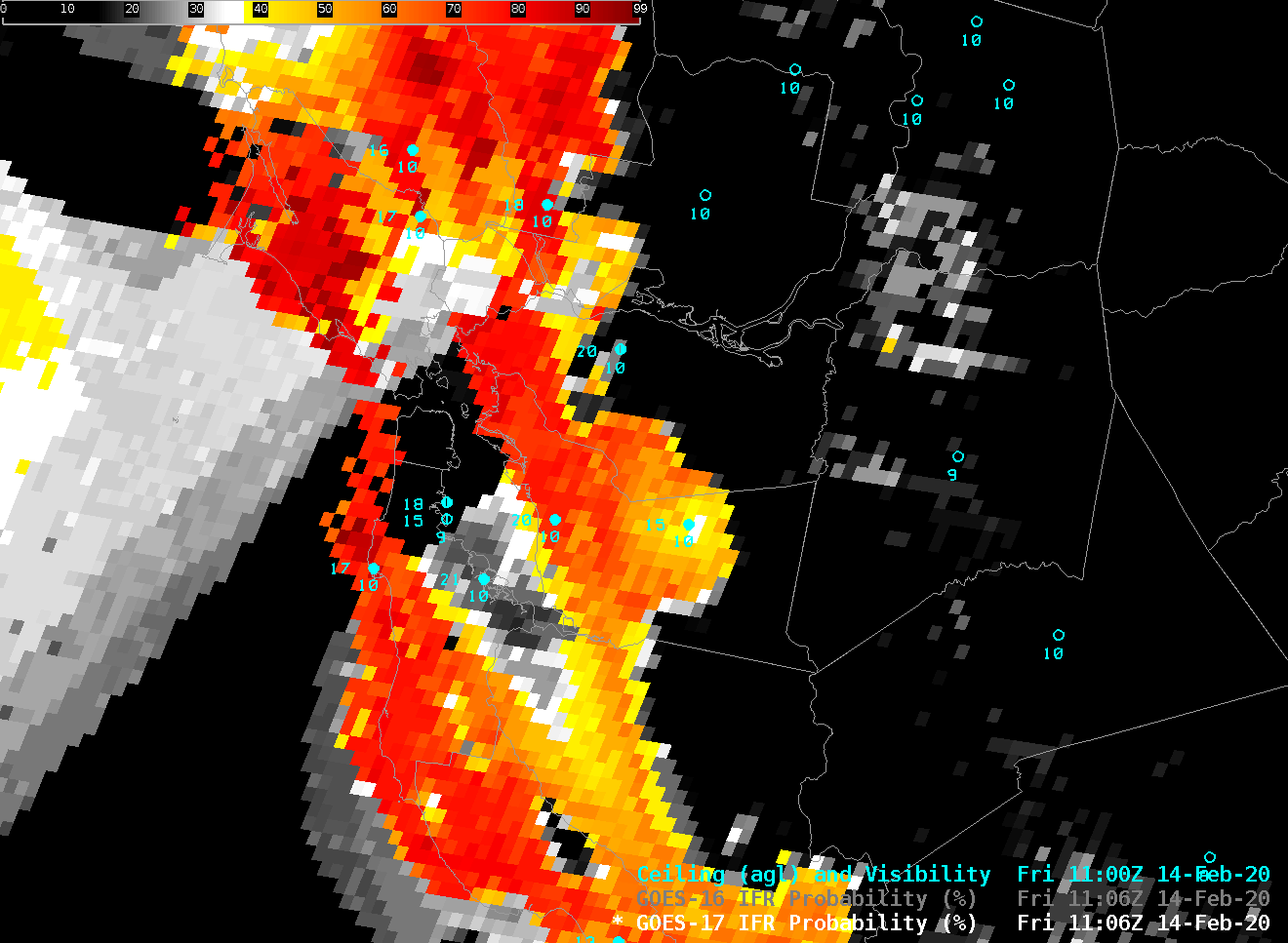
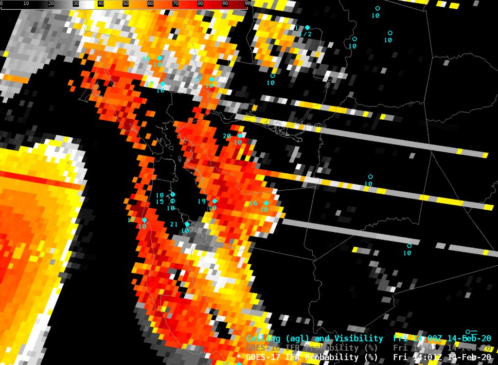
Because IFR Probability includes both model information on low-level saturation and satellite information on low-level clouds, it can give an advanced warning on the development of fog when high clouds — at might occur behind departing convection, for example — prevent the satellite from viewing the low cloud beneath high clouds.  Consider the animation below, that shows IFR Probability fields along with surface observations of ceilings and visibilities plotted so that regions with IFR conditions can be identified.  IFR probability fields develop over northwest Indiana over the course of the night, especially over extreme northern Indiana where the east-west Indiana Toll road sits.

GOES-R IFR Probability fields, along with observations of ceilings and visibility, 0051 – 1321 UTC (every 10 minutes) on 3 August 2020 (Click to enlarge)

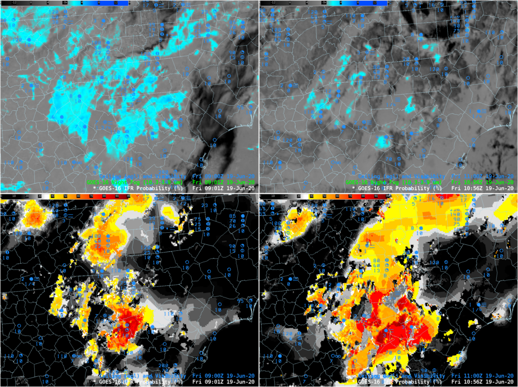
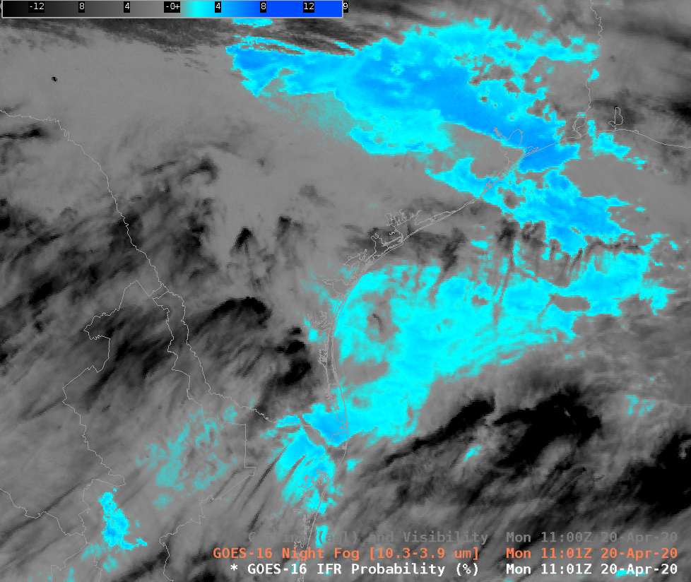
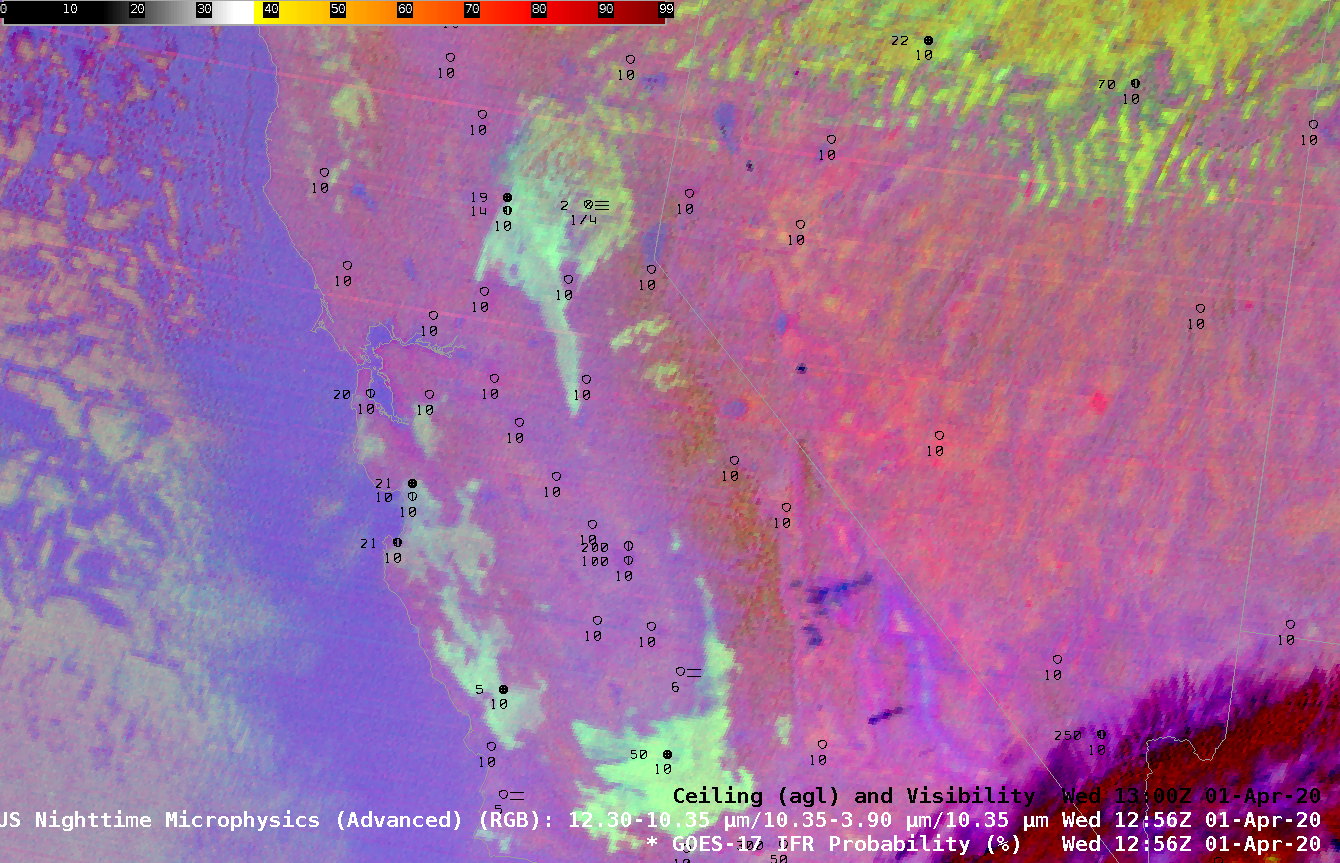
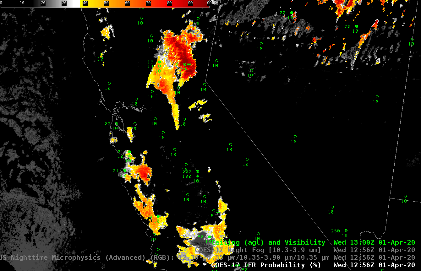
Compare the IFR Probability fields above to the Night Fog Brightness Temperature Difference (10.3 µm – 3.9 µm) field below. The field below historically has been used at night to identify regions of low clouds/fog — regions that are cyan in the enhancement are low clouds, regions that are black are high clouds. As the sun rises, the Night Fog brightness temperature difference field will struggle to identify regions of low clouds (although a different enhacement can be used to highlight the low cloud regions after sunrise). The satellite is not able to view low clouds over northern Indiana until the high clouds move out. Thus, a distinct indication of low clouds over the Indiana Toll road lags the suggestion of low clouds given by IFR Probability fields.

GOES-16 ‘Night Fog’ Brightness Temperature Difference (10.3 µm – 3.9 µm), every ten minutes from 0051 to 1321 UTC, 3 August 2020 (click to enlarge)

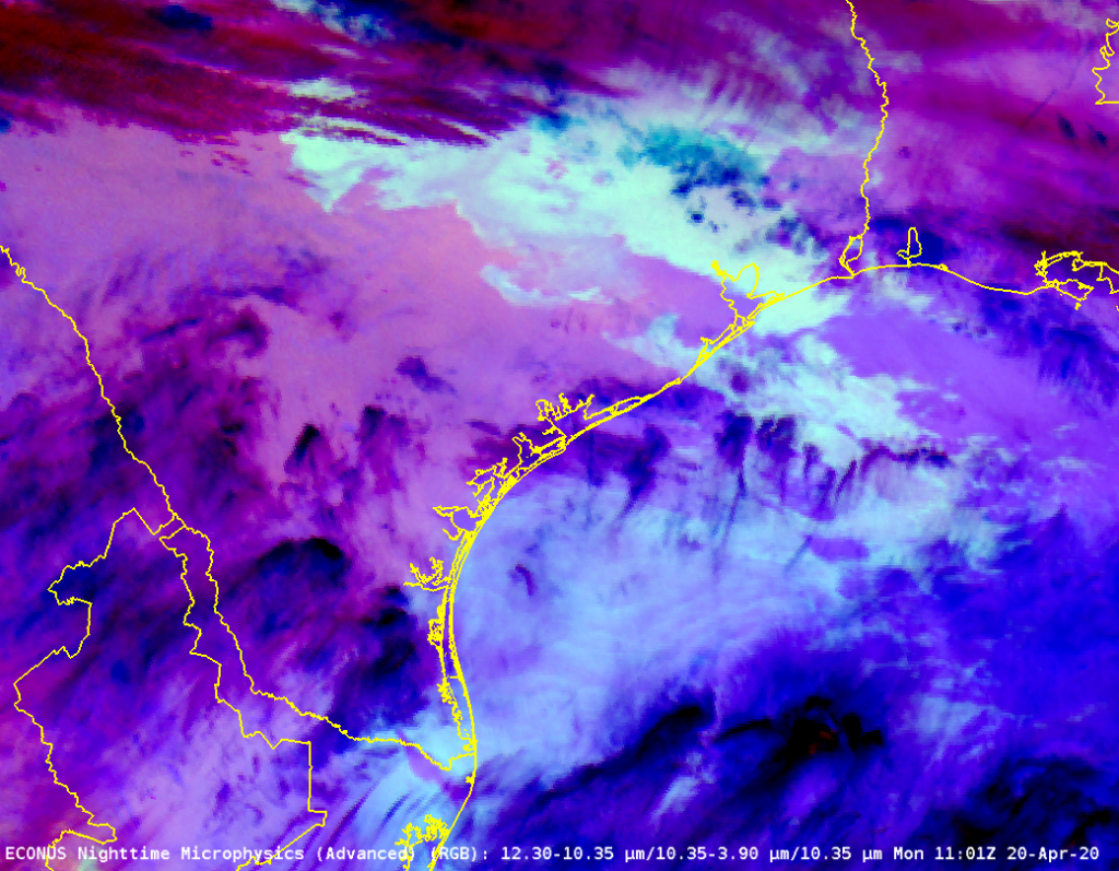
Consider the toggle below of GOES-R IFR Probability, Night Fog Brightness Temperature Difference and the Nighttime Microphysics RGB at 0601 UTC on 3 August.. IFR Probability fields show a developing region of IFR conditions (in yellow) over extreme NW Indiana. The two satellite-only detectors show only a scant suggestiong that fog is present. (A similar scenario is occurring near the bootheel of Missouri)

GOES-R IFR Probability, Night Fog Brightness Temperature Difference (10.3 µm – 3.9 µm), and Nighttime Microphysics RGB, 0601 UTC on 3 August 2020 (Click to enlarge)

At 0901 UTC, below, all three indicators of low clouds are in better agreement over northwest Indiana (and over the Missouri Bootheel) as high clouds move from those areas.

GOES-R IFR Probability, Night Fog Brightness Temperature Difference (10.3 µm – 3.9 µm), and Nighttime Microphysics RGB, 0901 UTC on 3 August 2020 (Click to enlarge)

Fields at 0931 and 1001 UTC continue this trend of stronger signals in the regions initially highlighted at 0601 UTC by the IFR Probability fields.

GOES-R IFR Probability, Night Fog Brightness Temperature Difference (10.3 µm – 3.9 µm), and Nighttime Microphysics RGB, 1031 UTC on 3 August 2020 (Click to enlarge)

By 1131 UTC, below, increasing solar reflectance over the eastern part of the domain has changed the signal in both the Nighttime fog and Nighttime microphysics RGB over northern Indiana and Ohio. The GOES-R IFR Probability signal however is maintained.

GOES-R IFR Probability, Night Fog Brightness Temperature Difference (10.3 µm – 3.9 µm), and Nighttime Microphysics RGB, 1131 UTC on 3 August 2020 (Click to enlarge)

Assessing IFR probabilties in regions with multiple cloud layers: San Francisco on 24 June 2020

GOES-17 ‘Night Fog’ Brightness Temperature Difference (10.3 µm – 3.9 µm) 0941 UTC – 1436 UTC, 24 June 2020 (Click to enlarge)

GOES-17 ‘Night Fog’ Brightness Temperature Difference imagery, above, shows a stratus deck (cyan and blue in this default AWIPS enhancement) off the central California coast. Higher clouds (grey and black in the enhancement) are drifting over San Francisco bay, obscuring the GOES-17 satellite’s view of low clouds. These high clouds can present a challenge to aviation forecasters for San Francisco’s airport, and important airline hub because the nature of low clouds cannot be determined. (Note the striping in the image is an artifact of GOES-17’s malfunctioning Loop Heat Pipe). This animation also shows the effect of increasing amounts of reflected solar radiation on the Night Fog Brightness Temperature Difference signal.

GOES-17 IFR Probability fields, below, augment information at low levels by using model (Rapid Refresh) estimates of low-level saturation (as might be found in low stratus) in the computation of IFR Probability. The animation below shows that SFO was in a region of high — but not very high — IFR Probabililty. Note also how the signal is constant through the sunrise at the end of the animation.

The airport (KSFO) did not report IFR conditions on this morning.

GOES-17 IFR Probability fields, 0941 – 1436 UTC, 24 June 2020 (Click to enlarge)

Morning IFR Conditions over South Carolina

Fog developed over North and South Carolina (some of this region has been cloudy and wet for much of the past week; here is a weekly precipitation total from this site) on the morning of 19 June 2020; the screenshot above, from this site, shows a sigmet related to the IFR conditions present:

How did GOES-R IFR Probability capture this event? The animation below, from 0900 to 1306 UTC, shows generally high IFR Probabilities over most of the region. There are stations where IFR conditions are occurring and IFR Probabilities are low: the Columbus County Municipal Airport (KCPC, in southeast North Carolina), for example, shows obstructed ceilings and reduced visibility. This might be a localized sub-pixel scale fog related to the small streams near the airport there. A similarly small-scale fog event may be happening at Macon County airport (K1A5) in western North Carolina. The 0901 UTC Brightness Temperature Difference field shows a signal consistent with valley fog along the Little Tennessee River (see image at bottom)

Note how the signal shows little discernible impact from the rising of the Sun. A strength of this product is that uniformity — in contrast to the Night Fog Brightness Temperature difference field.

GOES-16 IFR Probabilities, 0901 UTC – 1306 UTC on 19 June 2020. Surface observations of ceilings and visibilities shown in blue (Click to enlarge)

The 4-panel image below shows the ‘Night Fog’ Brightness Temperature Difference (10.3 µm – 3.9 µm, top) at 0901 and 1056 UTC and the IFR Probability fields, also at 0901 and 1056 UTC. IFR probability shows an expansion in the region of low ceilings reduced visibilities, as might be expected to occur around sunrise. The Night Fog Difference field shows a decrease in signal related to the increasing amount of reflected 3.9 µm solar insolation.

Night Fog Brightness Temperature Difference (10.3 µm – 3.9 µm), top and GOES-R IFR Probability, bottom, both at 0901 UTC (let) and 1056 UTC (right) on 19 June 2020.

Dense Fog over Virginia

GOES-16 Night Fog Brightness temperature Difference (10.3 µm – 3.9 µm), Night time Microphysics RGB and IFR Probability fields, 0801 UTC on 27 May 2020. Plots of ceilings and visibilities are included (click to enlarge)

Dense Fog was widespread over southeast Virginia on 27 May 2020. The toggle above compares the Night Fog Brightness Temperature Difference field, Night Time Microphysics RGB, and GOES-R IFR Probabilities computed with GOES-16 data and Rapid Refresh Model output, all at 0801 UTC. A challenge with satellite-only detection of low ceilings/poor visibility is that high clouds get in the way. For example, consider the satellite-only signal at Richmond, with 1/4-mile visibility and 200-foot ceilings. Low clouds are not easily detected in that region by satellite; only the GOES-R IFR Probability field (which blends satellite detection of clouds with model estimates of low-level saturation) correctly suggests the transportation hazard that is present there (and extending some distance to the north and west!)

GOES-16 Night Fog Brightness Temperature Difference (10.3 µm – 3.9 µm) field, 0701-1326 UTC on 27 May 2020 (Click to enlarge)

The animation of the night Fog brightness temperature difference field, above, the ‘green’ component of the night time microphysics RGB, shown below, shows a second challenge of using this product for fog detection: the signal is lost (or, at best, changes) as the Sun rises. The RGB product shows the same challenges in fog/low stratus detection that are present in the channel difference field above: high clouds mask the signal, and the signal changes as the sun rises. (Contrails show up very nicely in both however.)

GOES-16 Night Fog Microphysics RGB, 0701 – 1326 UTC on 27 May 2020 (Click to enlarge)

GOES-R IFR Probability fields, below, do a much better job characterizing the horizontal extent of the low clouds early in the animation, and in highlighting the region where visibility reductions persist through sunrise, namely from Hampton Roads northeastward along the coast.

GOES-16 IFR Probability fields, 0701-1326 UTC on 27 May 2020 (Click to enlarge)

IFR conditions over the Great Plains

Surface Analysis at 0900 UTC on 13 May 2020

Much of the central Plains of the United States was under easterly flow during the night on 12-13 May 2020, as suggested by the surface analysis above. Strong High Pressure over the Great Lakes and lower pressures over the Rocky Mountains drove that upslope flow. Consequently, IFR conditions were common over much of the Plains, as shown below.

The animation, below, of IFR Probability (overlain with surface observations and ceilings and visibilities) shows high probabilities. There is good correlation between regions with High IFR Probabilities — red and orange — and regions with low ceilings and reduced visibilities. The highest probabilities, dark red in the enhancement, occur where satellite data shows low clouds and where model data shows low-level saturation. Note that there is a trend towards less satellite information in the IFR Probability field with time over central Oklahoma and south-central Kansas because of developing convection.

GOES-16 IFR Probability fields, 0800-1136 UTC on 13 May 2020

The night time microphysics RGB, shown below, is also used to detect regions of low clouds; they typically appear yellowish at this time of year. The challenge with the RGB use in highlighting IFR conditions is two-fold: high clouds will mask the low cloud signal (as in the case of developing convection over Oklahoma, or with cirrus over Colorado and Nebraska). The RGB can also struggle to differentiate between fog and low stratus. Note also in this animation how the effect of the rising sun becomes apparent at the end of the animation over the eastern third of the image.

Night time Microphysics RGB, 0801-1136 UTC on 13 May 2020

In the toggle below, the signal of low clouds in the RGB, yellow/cyan over the Texas panhandle (for example) has an echo in the IFR Probability field. In the absence of high clouds, both products will show regions of low clouds. The Night Time Microphysics RGB gives extra information about the cloud type in regions where high clouds are blocking the satellite view of low clouds (the purple region over Colorado/Nebraska and the reddish regions over Kansas and Oklahoma). In contrast, the IFR Probabilty field in those regions gives no information on the character of the higher cloud; the IFR Probability field in those regions is flat (i.e., not pixelated), the hallmark of IFR Probability that is derived chiefly from model fields, so all an analyst can tell is that a high cloud is present.

GOES-16 IFR Probability and Night Time Microphysics RGB, 1001 UTC on 13 May 2020

IFR Probability with a frontal passage over Pennsylvania

GOES-16 ABI Band 2 (0.64 µm) Visible Imagery, 1000-1700 UTC on 11 May 2020

Frontal passage with extratropical cyclones will frequently be accompanied by low ceilings and reduced visibilities, that is, IFR conditions. A loop of visible imagery, above, suggests a surface cyclone (surface analyses are shown below) but it is difficult to determine from the imagery where low ceilings and reduced visibilities are present. Continue reading

Sea Fog near Corpus Christi

GOES-16 ABI Band 02 (0.64 mm “Red Visible”) visible imagery, 1201-2311 UTC on 20 April 2020

GOES_16 Visible imagery, above (along with surface observations of ceilings and visibilities), shows fog and low clouds over south Texas and offshore waters. The observations plotted can allow you to determine where IFR conditions are apparent — where visibilities are between 1 and 3 statute miles and ceilings are between 500 and 1000 feet. It’s difficult to determine the area of IFR conditions based solely on cloud cover however.

The animation below shows the probability of IFR conditions, a product that fuses satellite information with low-level saturation information from the Rapid Refresh model (Click here for an animation with no observations). The morning fog over east Texas burns off fairly quickly, and only dense sea fog is left after about 1700 UTC (10 AM CDT). In many offshore regions (and over east Texas before sunrise), the IFR Probability field has a flat character to it that is typical of a IFR Probability field determined mostly by model data. More pixelated data (and somewhat higher probabilities) occur where breaks in the cloud allow for satellite data to identify low clouds.

GOES-R IFR Probability, 1101 UTC to 2311 UTC on 20 April 2020

The night fog brightness temperature difference field, below, highlights a challenge in identifying low clouds using satellite data alone (in contrast to the IFR Probability above that uses satellite and model data, fusing the strengths of both). When cirrus is present, it can mask the satellite’s view of the low cloud beneath. In addition, the Night Fog Brightness Temperature difference product is not consistent through sunrise, as the emissivity differences that drive the signal at night time (small cloud droplets are not black body emitters of 3.9 µm radiation, but they are blackbody emitters of 10.3 µm radiation) become overwhelmed by reflectivity differences during the day when far more 3.9 µm solar radiation is reflected than 10.3 µm solar radiation. Thus, in the day, both low clouds and high clouds show up as black in this enhancement: they are both able reflectors of 3.9 µm radiation.

Night Fog Brightness Temperature Difference (10.3 µm – 3.9 µm) fields from 1101 UTC to 2311 UTC on 20 April 2020

The Day Fog Brightness Temperature Difference field, below, shows how cirrus ice crystals are initially more reflective of solar radiation, but as the sun climbs higher in the sky, low clouds start to reflect just as much solar radiation.

Day Fog Brightness Temperature Difference (3.9 µm – 10.3 µm) fields from 1201 UTC to 2311 UTC on 20 April 2020
GOES-16 Night Fog Brightness Temperature Difference (10.3 µm – 3.9 µm), 1101 UTC on 20 April 2020

The Night Fog Brightness Temperature Difference field, above, is a key component (the ‘green’ part) of the Advanced Night Time Microphysics RGB, shown below. Where the Brightness Temperature Difference field is unable to view low clouds, similarly the Night Time Microphysics RGB will be unable to highlight them.

GOES_16 Night Fog Microphysics, 1101 UTC 20 April 2020

Thanks to Penny Harness, WFO Corpus Christi, for alerting us to this event. (Link)

Detecting low ceilings over California

GOES-17 Night Fog Brightness Temperature Difference (10.3 µm – 3.9 µm) and Night Time Microphysics RGB, 1256 UTC on 01 April 2020 (Click to enlarge)

Detecting stratus at night, and thereby inferring the presence of fog, usually involves the Night Fog Brightness Temperature Difference (10.3 µm – 3.9 µm) field that identifies clouds made up of water droplets owing to the droplets’ different emissivity properties at 10.3 µm (droplets emit energy at that wavelength mostly as a blackbody) and at 3.9 µm (droplets do no emit energy at that wavelength as a blackbody). This difference field is a crucial component in the Night Time Microphysics Red-Green-Blue (RGB) Product as evinced in the toggle above. The regions shown to have low clouds (blue and cyan in the Brightness Temperature Difference field, pale yellow in the RGB) are not necessarily those regions with IFR conditions, i.e., where fog and low ceilings are present. The satellite can sense the top of the cloud, but it is a challenge to infer from the satellite data alone where the cloud base sits.

GOES-R IFR Probability fields combine satellite information with model estimates of low-level saturation. An accurate model simulation can allow the product to highlight regions of low ceilings (where fog is more likely) and screen out mid-level stratus. Consider the toggle below, and note how is emphasizes regions where observations show low ceilings and/or reduced visibilities (Blue Canyon airport northwest of Lake Tahoe and Paso Robles airport). Note also how the signal at Bakersfield, at the southern end of California’s Central Valley, is de-emphasized.

GOES-R IFR Probability fields provide a consistent signal for low ceilings and reduced visibility. The fields marry the strengths of satellite detection and model data.

GOES-17 Night Fog Brightness Temperature Difference (10.3 µm – 3.9 µm), GOES-17 IFR Probabilities, and GOES-17 Night Time Microphysics RGB, 1256 UTC on 01 April 2020 (Click to enlarge)

GOES-17 IFR Probability over San Francisco

GOES-17 IFR Probability over San Francisco, 1106 UTC, 14 February 2020, along with surface observations of ceilings and visibility (Click to enlarge)

The Cooperative Institute for Meteorological Satellite Studies (CIMSS) is (as noted in this blog post) testing GOES-17 IFR Probability fields in the AWIPS environment in preparation for their deployment to interested offices (via an LDM feed). The GOES-17 field, above, at 1106 UTC, suggests stratus offshore of San Francisco but higher ceilings over the city and the bay. Webcam views of the city (source), and of Alcatraz Island (source), below, from around 630 AM PST, also suggest relatively high ceilings over the city and the bay.

Webcam view of Alcatraz Island in San Francisco Bay, ca. 6:30 AM PST 14 February 2020

GOES-16 is also providing IFR Probability over the west coast of the United States. The toggle below between GOES-17 and GOES-16 shows how the oblique view from GOES-16 and the effects of parallax can perhaps place the probability in the wrong place. Parallax errors shift the clouds towards the sub-satellite point. Parallax effects can be explored at this website.

GOES-17 and GOES-16 IFR Probability fields, 1106 UTC on 14 February 2020 (Click to enlarge)

The GOES-17 Advanced Baseline Imager (ABI) is currently showing the effects of inadequate imager cooling by the faulty Loop Heat Pipe on board the spacecraft. At times between 1100 and 1500 UTC, as shown below for 1401 UTC, stripes will appear in the IFR Probability field. Manifestations of the Loop Heat Pipe issue will continue with increasing impact into early March, at which time Eclipse Season will mitigate the issue until April.

GOES-17 IFR Probability over San Francisco, 1401 UTC, 14 February 2020, along with surface observations of ceilings and visibility (Click to enlarge)

GOES-17 IFR Probability fields are available over the CONUS domain at this website.