")
GOES-15 0.62 µm Visible Imagery (Click to see animation)
It can be challenging to determine where fog and low stratus are problematic over Alaska. The visible imagery, above, shows an abundance of clouds (and, over the Northwest Territores, smoke) — but it’s difficult to guess which of the clouds are associated with low stratus or fog and accompanying low visibilities. Knowing where visibilities are low is vital in a state like Alaska where small aircraft provide vital transportation services.
After dark, increasingly frequent at this time of year in Alaska, the brightness temperature difference field (between brightness temperatures at 10.7 µm and 3.9 µm) can be used to identify water-based clouds because of differences at those two wavelengths in the emissivity properties of liquid water droplets that make up clouds. That animation is shown below. As with the visible imagery, the brightness temperature difference tells you about the top of the cloud. The important visibility restrictions occur at the bottom of the cloud.
 (Click to see animation)")
GOES-15 Brightness Temperature Difference (10.7 µm – 3.9 µm) (Click to see animation)
")
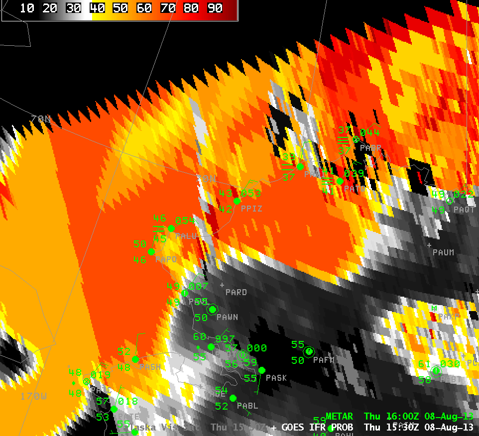
GOES-R IFR Probabilities computed from GOES-15 and Rapid Refresh Data (Click to see animation)
Neither the visible nor brightness temperature difference loops above highlight cloudy regions with restricted visibility. The GOES-R IFR Probability product that fuses satellite information with model output, a loop of which is available above, does. Many offshore regions show high probabilities of IFR conditions. These are likely regions of advection fog where relatively moist air is flowing over cold ocean waters and being cooled to its dewpoint. (Click here to see a surface plot over northwest Alaska — dewpoints are in the 40s and 50s near the Bering Sea) An area of high IFR probabilities that occurs over land is over southwest Alaska between Dillingham and Bethel. Dillingham does report IFR and near-IFR conditions as the higher IFR probabilities rotate through. A close-up image of the IFR Probability, hourly, over southwest Alaska is shown below; note how ceilings and visibilities in Dillingham (PADL) lower as the IFR probabilities increase.
")
GOES-R IFR Probabilities computed from GOES-15 and Rapid Refresh Data (Click to see animation)
VIIRS data from Suomi/NPP can also be used to approximate where fog may occur. Both the Day/Night band and the Brightness Temperature Difference product can tell a forecaster where clouds exist. However, surface conditions beneath the clouds detected by Suomi/NPP may or may not be consistent with IFR conditions. In the animation below, a new algorithm has been applied to the Day/Night band to extract information in the transition zone between day and night. Some artifacts of that algorithm are evident (manifest as what appear to be cloud bands perpendicular to the satellite path), but useful information about clouds do appear elsewhere. The brightness temperature difference product is only computed where solar reflectance is essentially nil. GOES Imagery is included in the loop to show where sunrise has occurred.
")
Suomi/NPP Day/Night band, Brightness temperature difference, and GOES Imager visible data, all near 1245 UTC on 8 August 2013 (Click to see animation)
")
")
 (Click to see animation)")
")
")
")
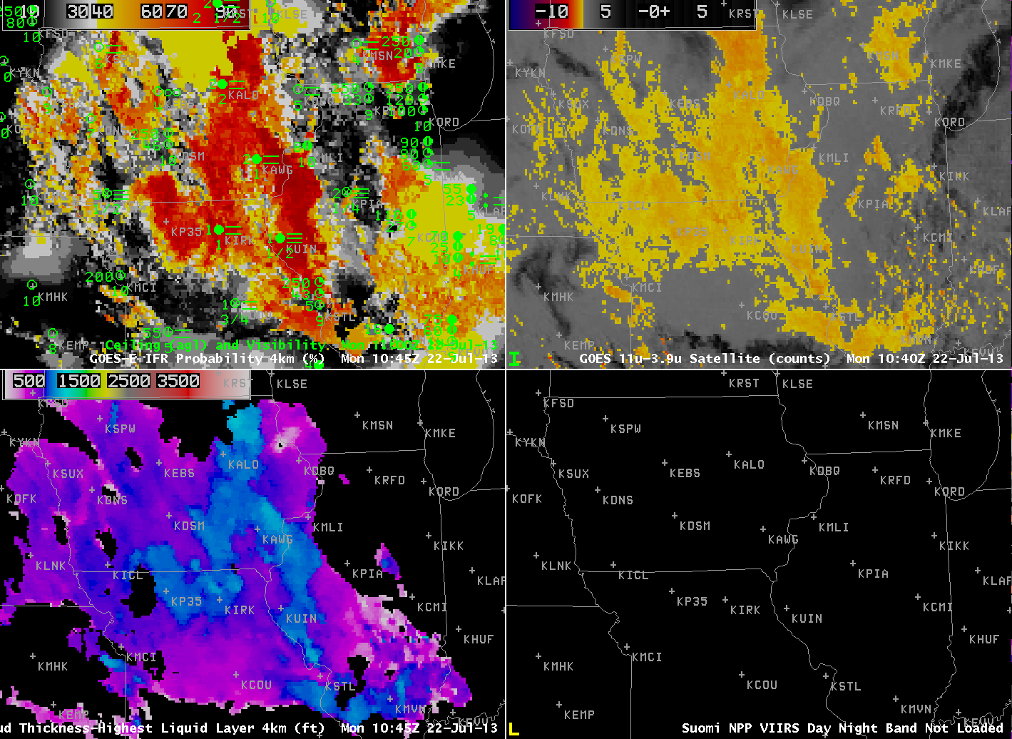
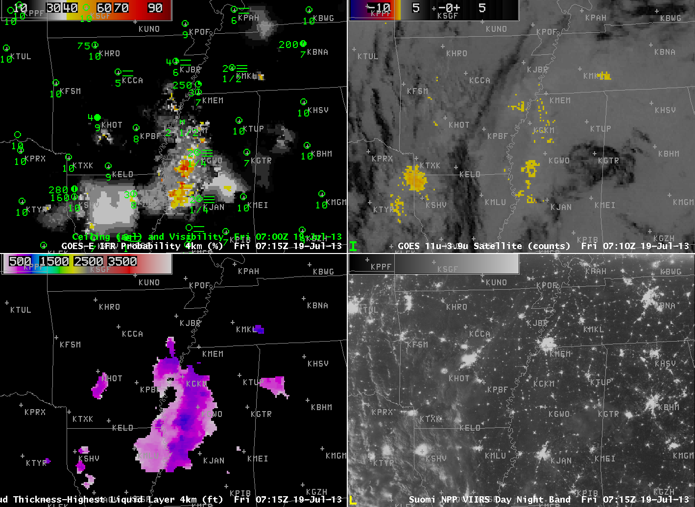
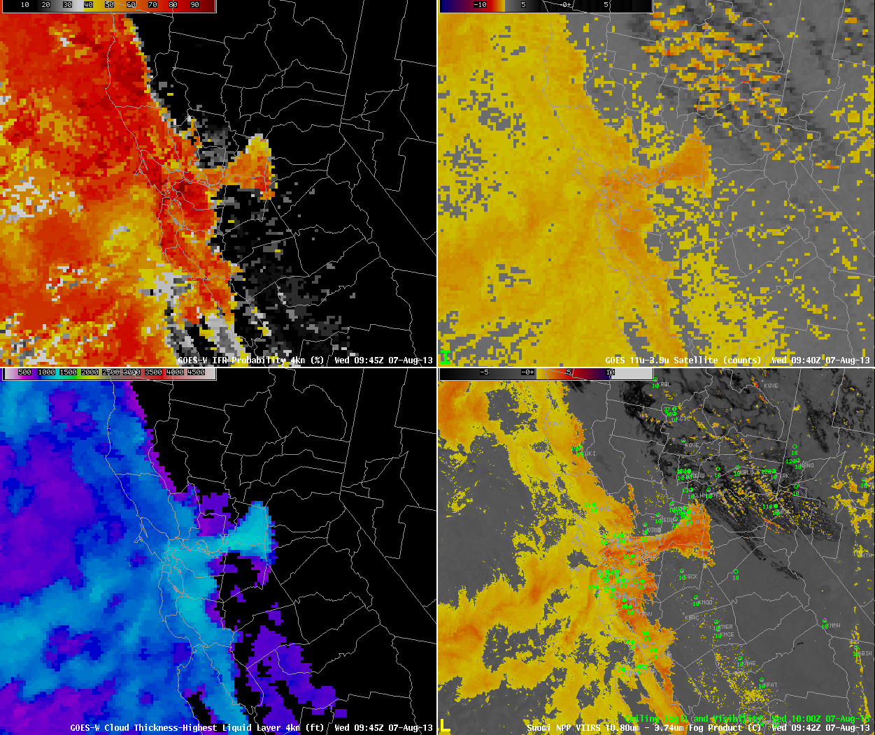
, GOES-West Brightness Temperature Difference (Upper Right, 10.7 µm - 3.9 µm), GOES-R Cloud Thickness (Lower Left), Suomi/NPP Brightness Temperature Difference (click image to play animation)")
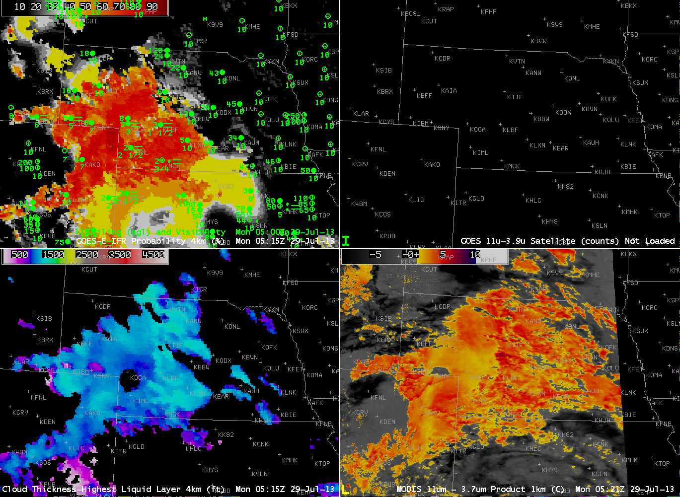
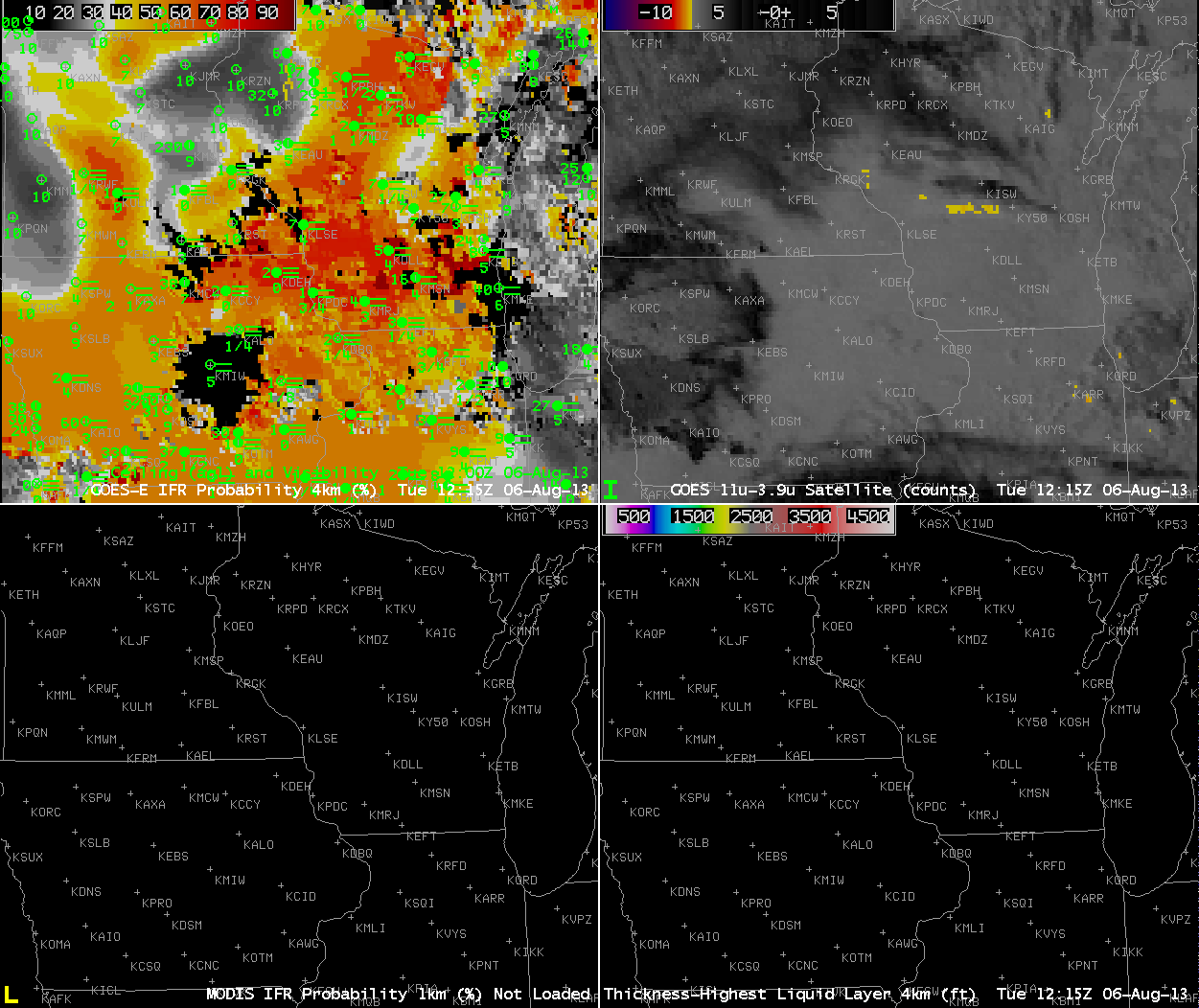
, GOES-East Brightness Temperature Difference (Upper Right, 10.7 µm - 3.9 µm), MODIS-based GOES-R IFR Probabilities (Lower Left), GOES-based GOES-R Cloud Thickness (Lower Right) (click image to play animation)")


