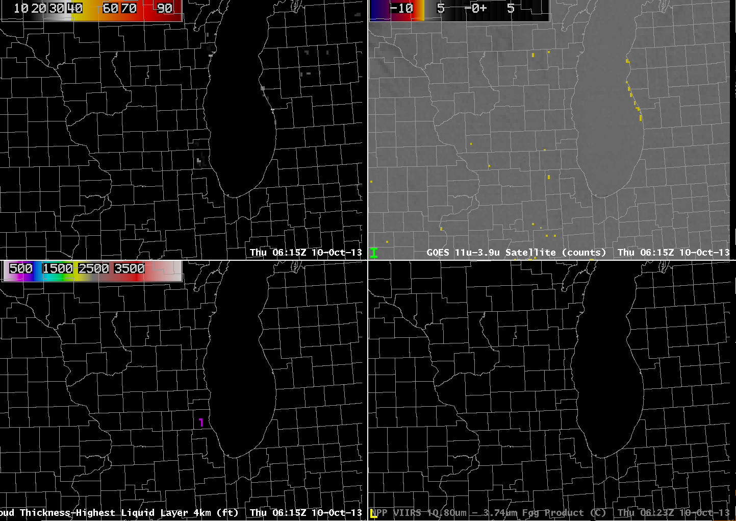
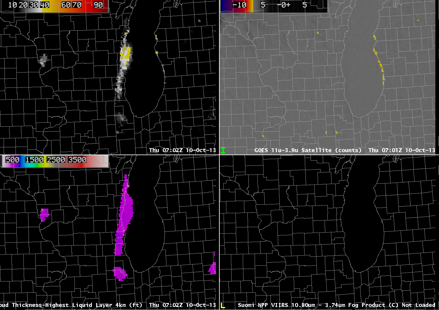
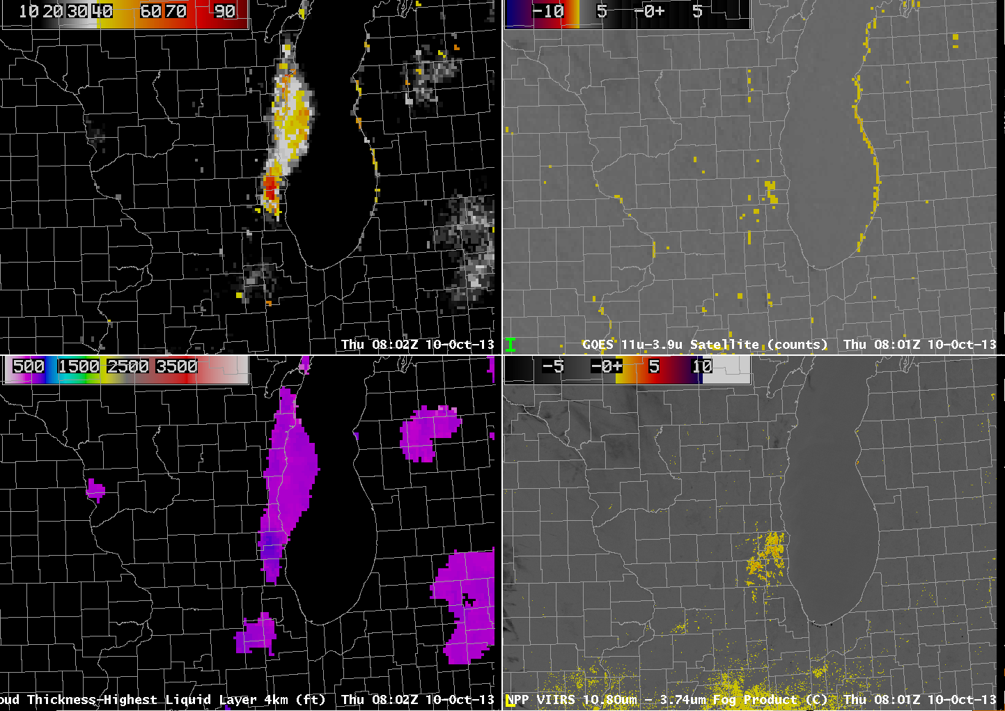
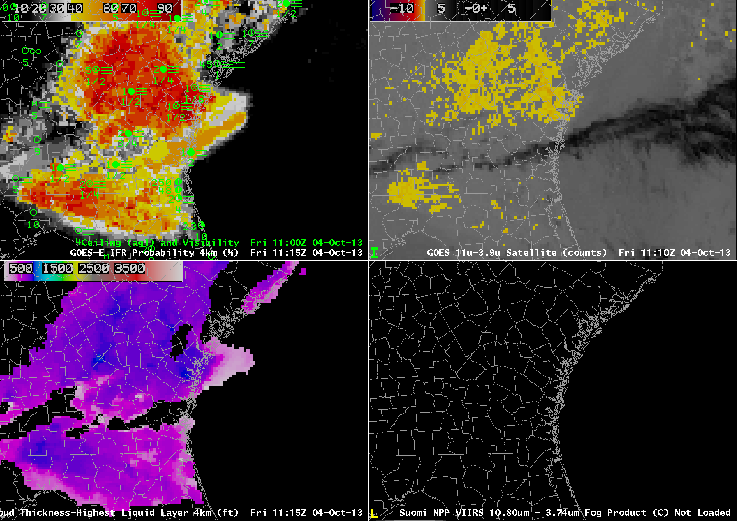
GOES-13-based GOES-R IFR Probabilities (Upper Left), GOES-13 Brightness Temperature Difference Product (10.7 µm – 3.9 µm) (Upper Right), GOES-R Cloud Thickness (Lower Left), Suomi-NPP Day/Night band (Lower Right), all times as indicated (click image to animate)
The ongoing change of seasons means that stronger large-scale weather systems are more likely. When something like a Colorado Cyclone moves from the Rockies and emerges into the central part of USA, it brings multiple cloud layers with it, and those many cloud layers make detection of fog and low stratus difficult. The animation above shows GOES-R IFR Probabilities and Cloud Thicknesses as well as the color-enhanced GOES-13 Brightness Temperature Difference (BTD) field. Note the characteristic signal in the BTD field of jet-level cirrus over Kansas. In these regions, BTD fields cannot be used to diagnose regions of low-level clouds because the upper-level clouds block the satellite view of lower clouds.
IFR Probability does have a signal over Kansas, however (where IFR conditions are present — see the animation below). Rapid Refresh data are being used under the cirrus to diagnose the probability of IFR conditions. Thus, IFR Probability fields are filled in under regions of high cirrus. Because only model data are being used to diagnose IFR Probability fields over central and southern Kansas, the characteristic of the field is different. Where satellite and model data are used, as over western Nebraska, the IFR Probability field has a pixelated appearance; where only model data are used, as over southern Kansas, the IFR probability field has a very smooth appearance. In model-only regions, in addition, IFR Probabilities are smaller because the number of predictors available to the algorithm is smaller.
The BTD field highlights regions in eastern Nebraska as having water-based clouds? Are these clouds causing low ceilings and reduced visibilities? No, and IFR probabilities in that region are low. In this region, Rapid Refresh data do not show low-level saturation, and thus the IFR Probabilities are correctly small, despite the strong satellite signal.
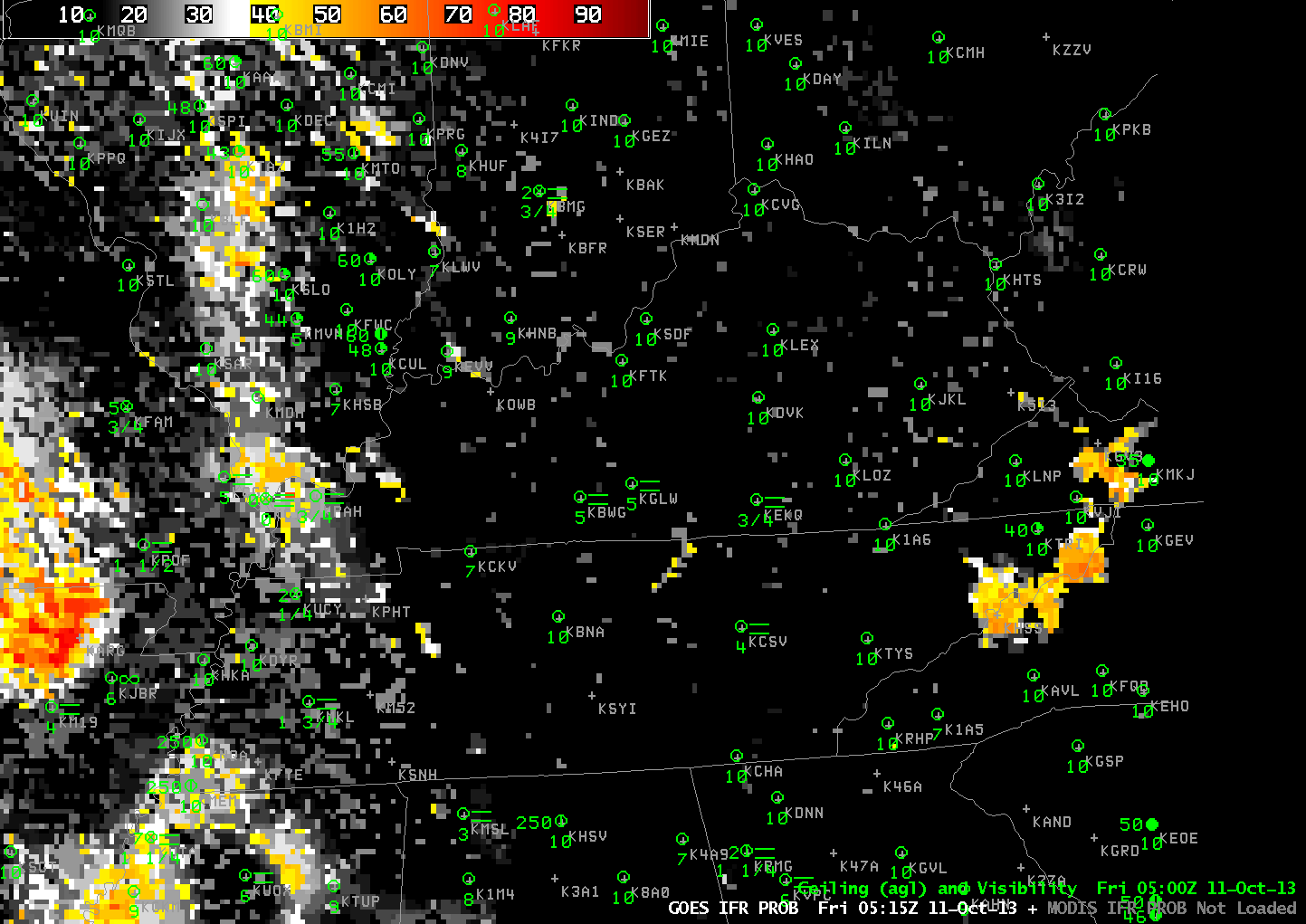
GOES-13-based GOES-R IFR Probabilities and surface visibilities/ceilings, all times as indicated (click image to enlarge)
GOES-R Cloud Thickness, shown at top, is only computed in regions where the highest cloud detected by the satellite is water-based; the algorithm considers includes information from a cloud-typing algorithm, and if clouds are ice phase (or mixed phase) as is likely in the case of jet stream cirrus, cloud thickness is not computed. (Cloud Thickness is also not computed during times of twilight — that is, an hour or so on either side of sunrise and sunset).
As above, but for a case of Stray Light, all times as indicated (click image to enlarge)
There are still cases at night when Stray Light will contaminate/enhance the 3.9 µm signal on GOES-13, and this contamination can propagate into the GOES-R IFR Probability of Cloud Thickness Fields. In this case, only the Cloud Thickness Fields are affected (below); Cloud thickness jumps about 500 feet for one time period (0415 UTC).
