Monthly Archives: August 2013

Northern Indiana Fog Event

VIIRS_DNB__REF_20130829_0748

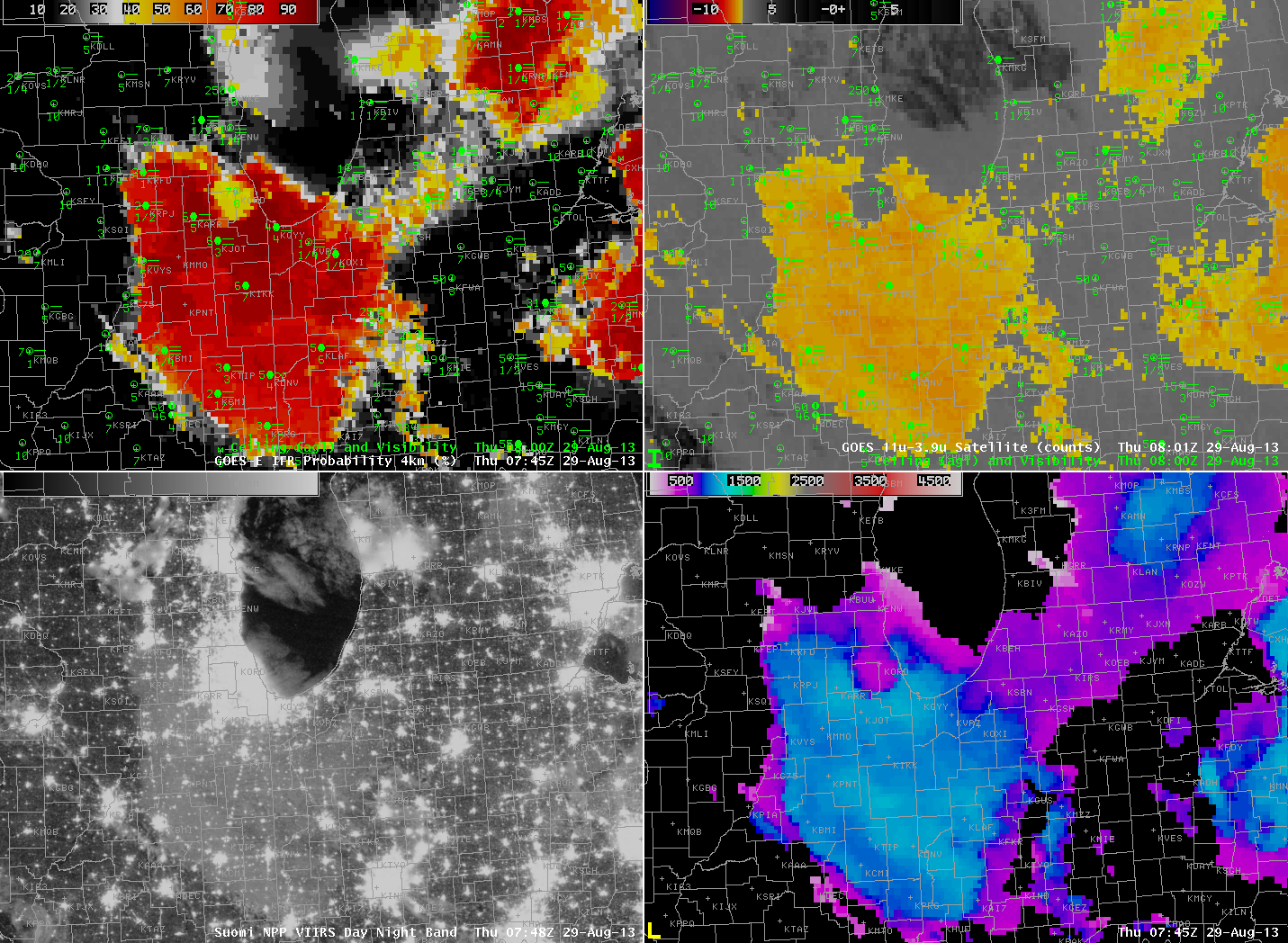
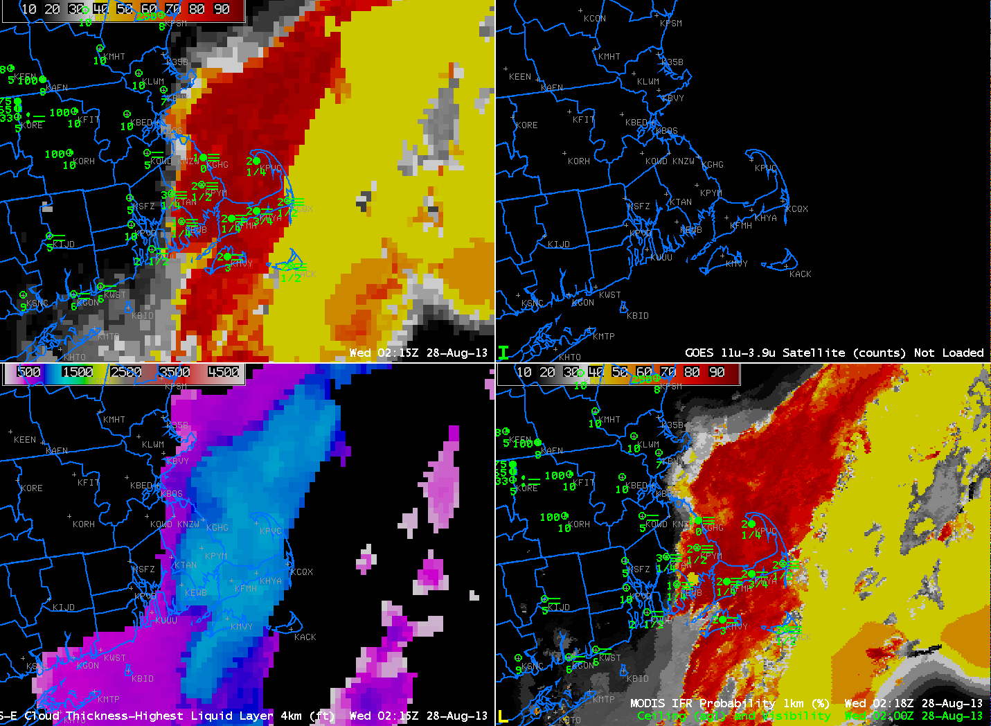
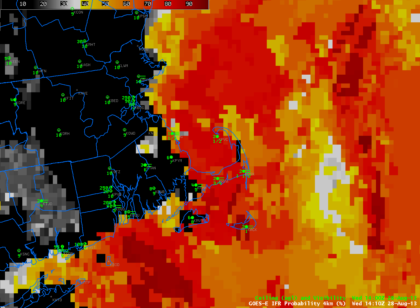
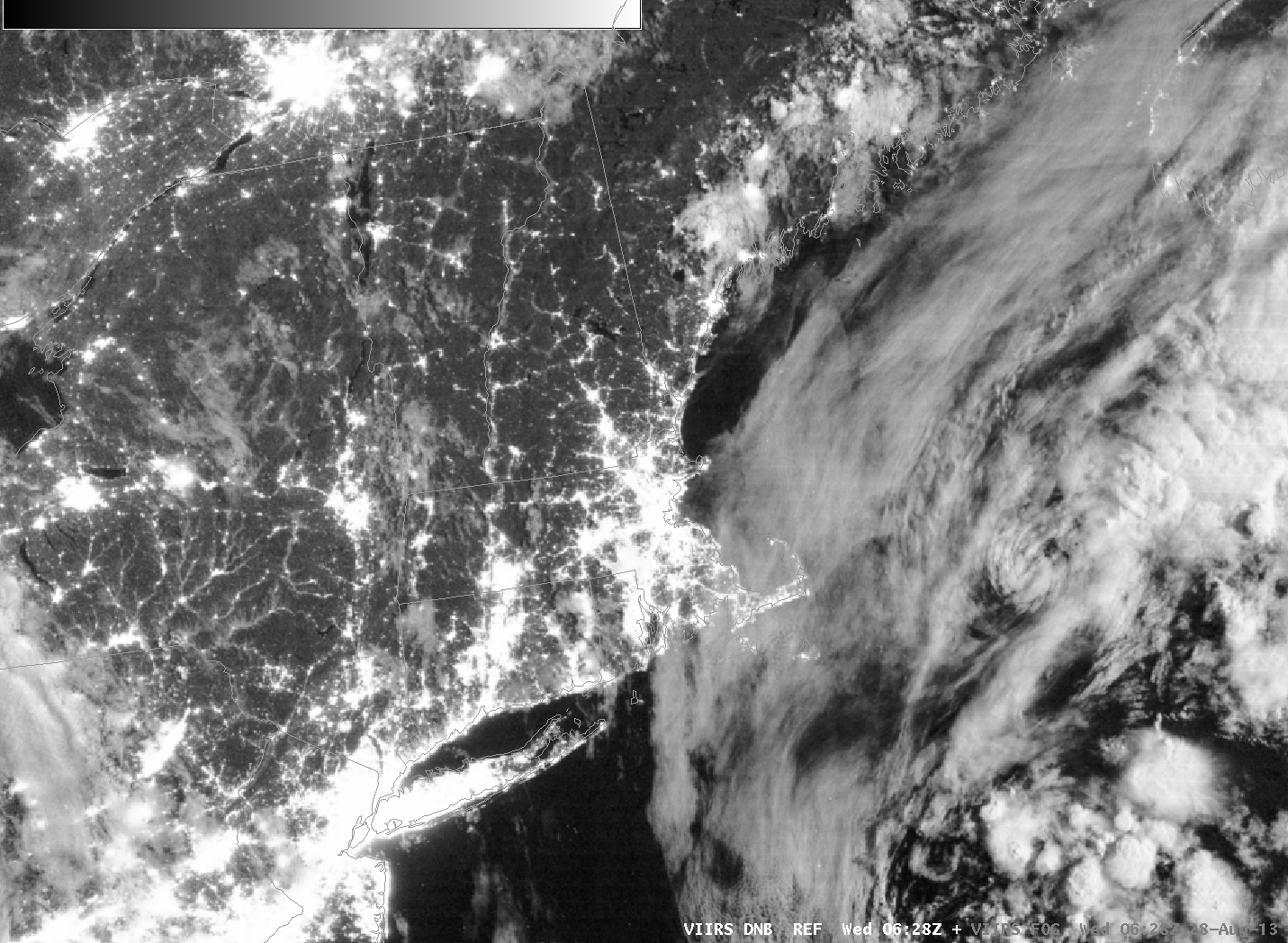
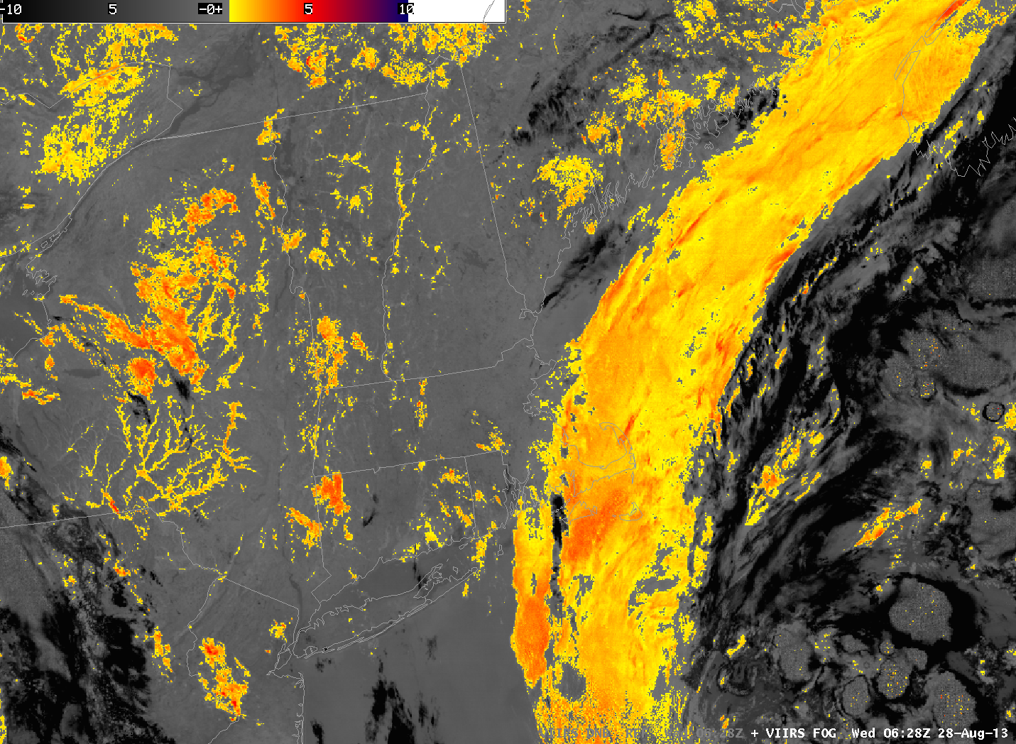
Dense fog developed overnight over NW Indiana and adjacent regions. The GOES-R IFR Probability Product highlighted the regions with the densest fog, refining somewhat the regions highlighted by the brightness temperature difference, the heritage fog-detection product. The image above shows the IFR Probability (Upper Left), Brightness Temperature Difference (Upper Right), Day/Night Imagery from Suomi/NPP (Lower Left) and GOES-R Cloud Thickness (Lower Right). Forecast offices were alert to the possibility of fog, as shown in AFDs from LOT (Chicago) and IWX (Northern Indiana)

000
FXUS63 KIWX 290619
AFDIWX

AREA FORECAST DISCUSSION
NATIONAL WEATHER SERVICE NORTHERN INDIANA
219 AM EDT THU AUG 29 2013

.SYNOPSIS…
ISSUED AT 137 AM EDT THU AUG 29 2013

AN UPPER LEVEL RIDGE WILL CONTINUE ACROSS THE MIDWEST…CAUSING
TEMPERATURES TO STAY MUCH ABOVE NORMAL WITH DRY CONDITIONS. HIGHS
TODAY AND FRIDAY WILL BE IN THE MID 80S TO LOWER 90S. LOWS TONIGHT
WILL BE AROUND 65 DEGREES.

&&

.UPDATE…
ISSUED AT 137 AM EDT THU AUG 29 2013

UPDATED THE GRIDS/FCST TO MENTION AREAS OF FOG DEVELOPING.
CLEARING SKIES OVER MUCH OF THE AREA COMBINED WITH RESIDUAL
MOISTURE AND LIGHT WINDS FAVOR FOG FORMATION. CURRENT THINKING IS
THE FOG EXPECTED TO BECOME WIDESPREAD BY LATE TONIGHT…AND WILL
PROBABLY BECOME DENSE IN AREAS. HAVE HELD OFF ON A DENSE FOG
ADVISORY TO TRY TO GET A BETTER IDEA WHERE THE FOG WILL FORM…
ESPECIALLY AS SOME CLOUDS LINGER OVER NRN INDIANA.

000
FXUS63 KLOT 290906
AFDLOT

AREA FORECAST DISCUSSION
NATIONAL WEATHER SERVICE CHICAGO/ROMEOVILLE IL
406 AM CDT THU AUG 29 2013

.DISCUSSION…
324 AM CDT

THE FORECAST CHALLENGES INCLUDE FOG IN THE NEAR TERM…THEN
INCREASING TEMPS AND THUNDERSTORM CHANCES FRIDAY…FOLLOWED BY A
COOL DOWN AND RETURN TO MORE SEASONABLE CONDITIONS TOWARD END OF THE
HOLIDAY WEEKEND.

GOES IMAGERY THIS MORNING SHOWS EXPANDING AREA OF STRATUS ACROSS
MUCH OF THE FORECAST AREA WITH SURFACE OBS AND WEBCAMS SHOWING A
SMATTERING OF DENSE FOG HERE AND THERE. ALL INDICATIONS ARE THAT THE
STRATUS IS THIN AND SHOULD BURN OFF QUICKLY THIS MORNING EXPECT NEAR
THE LAKE FRONT WHERE MARINE STRATUS AND POSSIBLY EVEN SOME FOG COULD
HOLD ON INTO THE AFTERNOON. ANOTHER COMPARATIVELY COOL DAY NEAR THE
LAKE WITH 70S RANGING QUICKLY UPWARD TO 80S INLAND JUST A FEW MILES
WITH UPPER 80S TO NEAR 90 EXPECTED SOUTHERN AND WESTERN PORTIONS OF
THE CWA.

GOES_IFR_PROB_20130829_0202.png

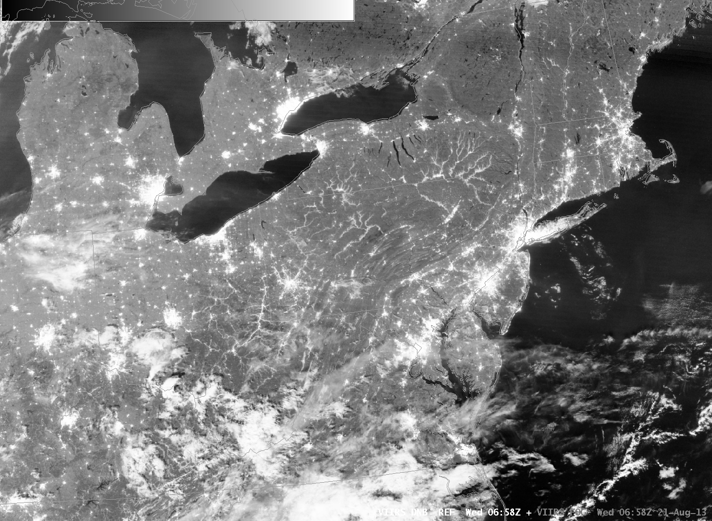
GOES-R IFR Probability (Upper Left), GOES-East Brightness Temperature Difference (Upper Right), Suomi/NPP Day/Night Band (Lower Left), GOES-R Cloud Thickness (Lower Right) (click image to play animation)

Aspects of the loop above require comment. Note that initially there is a region of enhanced brightness temperature difference over northern Indiana, between Fort Wayne (KFWA) and Muncie (KMIE), in a region where IFR conditions are not reported. The GOES-R IFR Probabilities in this region are very small (correctly), likely reflecting the influence of the Rapid Refresh model on the IFR Probability product. In other words, this is a region for which the model is not predicting low-level saturation, at least early in the evening. The Brightness Temperature Difference signal is likely a result of elevated stratus.

Later on in the animation, IFR probabilities start to increase between NW Indiana and Saginaw MI, a region where visibilities are decreasing but where the brightness temperature difference, initially, has little signal.

In this case, the IFR Probability Fields improved on the Brightness Temperature Difference predictions — suppressing a signal in regions of stratus, and developing a signal before a signal is present in the brightness temperature difference field alone. This is the power of a fused data product.

The IFR Probability field will also provide a consistent signal through sunrise.

Fog dissipation is shown in the animation below (Click the image to start the animation). Cloud thickness is especially thick over central Illinois, and fog was slow to burn off there. Stratus also persisted over southern Lake Michigan.

NWINFOG_29AUGloop

Fog on Cape Cod

Loop of IFR Probabilities

Fog developed over Cape Cod and the Islands overnight into the early morning on August 28th. The animation above (click image to animate) shows high IFR probabilities over land adjacent to the ocean. Observations show IFR or near-IFR conditions in these regions. IFR conditions decreased after sunrise. By 1410 UTC, the final image in the loop, IFR conditions persisted mostly only over Nantucket and Cape Cod east of Falmouth. This is where highest IFR probabilities persisted. The GOES-based IFR Probabilities suggest a sharp edge to the lowest visibilities over far eastern Massachusetts, which edge was just east of a Newport (RI) to Taunton (MA) line. MODIS-based IFR probabilities at 0218 UTC, below, also suggest a sharp western edge to the IFR conditions.

MODIS-based IFR Probabilities

VIIRS data from Suomi/NPP includes both the Day/Night Band and a Brightness Temperature Difference. These data are toggled with the GOES-based IFR Probabilities below. Resolution limitations inherent with GOES data preclude the accurate detection of fog in small river valleys.

Suomi/NPP Day/Night Band Imagery, Brightness Temperature Difference Imagery, and GOES-Based IFR Probabilities, all near 0630 UTC on 28 August

Valley Fog in Pennsylvania

VIIRS_20130821_0658

The above animation bewteen the Suomi/NPP VIIRS Day/Night Band and the brightness temperature difference between the longwave infrared image and the shortwave infrared image (that highlights water-based clouds because of emissivity differences at the two wavelengths) shows fog/low stratus in the river valleys of Pennsylvania. The high spatial resolution of Suomi/NPP allows remarkable detail, and the near-Full Moon provides ample illumination. How well did more conventional satellite imagery depict the developing fog? The GOES-13-based IFR Probability Field, below, shows relatively high values in regions over Pennsylvania that are near the river valleys, but GOES lacks the spatial resolution to portray adequately the horizontally confined river valley fog — although someone with knowledge of Pennsylvania Geography can infer a lot.

GOES_IFR_PROB_20130821_0702

The strength of GOES imagery is temporal consistency and 15-minute timesteps. Polar orbiter data can only give occasional looks. For example, MODIS Imagery can be used to generate brightness temperature differences and IFR Probabilities, below, but they are produced only every 90 minutes at most (although they will still give useful information, even at the edges of the MODIS swath where resolution is degraded).

MODIS_FOG_20130821_loop

MODIS_IFR_PROB_20130821_loop

The animation of IFR Probabilities from GOES-East, below, nicely depicts the slow increase in Valley Fog. This animation in concert with knowledge of the geography, augmented with the occasional high-resolution imagery from polar orbiters, as above, should allow a forecaster to describe the location of fog development overnight.

GOES_IFR_PROB_20130821_loop

Visible imagery, below, shows the dissipation of the fog during the morning of August 21st.

GOES13_VIS_21AUG2013loop

Fog was also abundant over Pennsylvania the morning of 20 August. GOES-14, in SRSO-R mode, captured the dissipation. Link. (Courtesy Dan Lindsey, NOAA).

What does MODIS-type Resolution get you?

MODIS-based IFR Probabilities and Cloud Thickness, 0657 UTC on 15 August 2013

MODIS-based IFR Probabilities and Cloud Thickness, 0657 UTC on 15 August 2013

The 1-km data available from the MODIS (above) that is on the Terra and Aqua satellites allows much better resolution than the nominal 4-km resolution from GOES-East and GOES-West (below). The higher resolution on MODIS yields better depiction of dendritic valley fog patterns in mountainous regions. Extremes in cloud thickness will be deeper with MODIS data as well. (In this example, MODIS-based cloud depths reach 1300 feet, vs. 900 feet in GOES) In addition, because fog/low stratus generally starts at small scales and grows in size, MODIS is more likely to detect the early stages of fog (if a serendipitous overpass occurs). Thus, a forecaster can be alert to subsequent development in the GOES data with its better temporal resolution.

GOES-based IFR Probabilities and Cloud Thickness, 0657 UTC on 15 August 2013

GOES-based IFR Probabilities and Cloud Thickness, 0702 UTC on 15 August 2013

1-minute Imagery of Fog Dissipation

GOES-14 0.62 µm Visible images (click image to play animation)

GOES-14 0.62 µm Visible images (click image to play animation)

GOES-14 is in experimental SRSO-R mode for the next few weeks, and the 1-minute imagery it is yielding provides a close look at the dissipation of fog after sunrise. In this example, fog in the Wisconsin River Valley burns off. How did ‘conventional’ observations of the fog produced from GOES-13 and the Rapid Refresh Model observe this small region of fog? Hourly imagery of IFR Probabilities, below, show the development of highest probabilities along the Wisconsin River. This is a region where IFR conditions were observed around sunrise.

GOES_IFR_PROB_20130814loop

GOES-R IFR Probabilities (click image to play animation)

GOES-R Cloud Thickness, below, also shows a signal over the Wisconsin River, with maximum cloud thickness around 800 ft. According to this chart, a fog with a thickness of 800 feet should burn off in between 1 and 2.5 hours. The GOES-14 animation confirms this prediction. Fog dissipates shortly after 1400 UTC. Note that the GOES-R Cloud Thickness loop, below, terminates at 1102 UTC, the last image before twilight conditions necessitate that the product not be computed.

GOES_CLD_THICK_20130814loop

GOES-R Cloud Thickness (click image to play animation)

GOES-14 views of Valley Fog in West Virginia on this same day are available here.

Late Summer Fog Detection over Alaska

GOES-15 0.62 µm Visible Imagery (Click to see animation)

GOES-15 0.62 µm Visible Imagery (Click to see animation)

It can be challenging to determine where fog and low stratus are problematic over Alaska. The visible imagery, above, shows an abundance of clouds (and, over the Northwest Territores, smoke) — but it’s difficult to guess which of the clouds are associated with low stratus or fog and accompanying low visibilities. Knowing where visibilities are low is vital in a state like Alaska where small aircraft provide vital transportation services.

After dark, increasingly frequent at this time of year in Alaska, the brightness temperature difference field (between brightness temperatures at 10.7 µm and 3.9 µm) can be used to identify water-based clouds because of differences at those two wavelengths in the emissivity properties of liquid water droplets that make up clouds. That animation is shown below. As with the visible imagery, the brightness temperature difference tells you about the top of the cloud. The important visibility restrictions occur at the bottom of the cloud.

GOES-15 Brightness Temperature Difference (10.7 µm - 3.9 µm) (Click to see animation)

GOES-15 Brightness Temperature Difference (10.7 µm – 3.9 µm) (Click to see animation)

GOES-R IFR Probabilities computed from GOES-15 and Rapid Refresh Data (Click to see animation)

GOES-R IFR Probabilities computed from GOES-15 and Rapid Refresh Data (Click to see animation)

Neither the visible nor brightness temperature difference loops above highlight cloudy regions with restricted visibility. The GOES-R IFR Probability product that fuses satellite information with model output, a loop of which is available above, does. Many offshore regions show high probabilities of IFR conditions. These are likely regions of advection fog where relatively moist air is flowing over cold ocean waters and being cooled to its dewpoint. (Click here to see a surface plot over northwest Alaska — dewpoints are in the 40s and 50s near the Bering Sea) An area of high IFR probabilities that occurs over land is over southwest Alaska between Dillingham and Bethel. Dillingham does report IFR and near-IFR conditions as the higher IFR probabilities rotate through. A close-up image of the IFR Probability, hourly, over southwest Alaska is shown below; note how ceilings and visibilities in Dillingham (PADL) lower as the IFR probabilities increase.

GOES-R IFR Probabilities computed from GOES-15 and Rapid Refresh Data (Click to see animation)

GOES-R IFR Probabilities computed from GOES-15 and Rapid Refresh Data (Click to see animation)

VIIRS data from Suomi/NPP can also be used to approximate where fog may occur. Both the Day/Night band and the Brightness Temperature Difference product can tell a forecaster where clouds exist. However, surface conditions beneath the clouds detected by Suomi/NPP may or may not be consistent with IFR conditions. In the animation below, a new algorithm has been applied to the Day/Night band to extract information in the transition zone between day and night. Some artifacts of that algorithm are evident (manifest as what appear to be cloud bands perpendicular to the satellite path), but useful information about clouds do appear elsewhere. The brightness temperature difference product is only computed where solar reflectance is essentially nil. GOES Imagery is included in the loop to show where sunrise has occurred.

Suomi/NPP Day/Night band, Brightness temperature difference, and GOES Imager visible data, all near 1245 UTC on 8 August 2013 (Click to see animation)

Suomi/NPP Day/Night band, Brightness temperature difference, and GOES Imager visible data, all near 1245 UTC on 8 August 2013 (Click to see animation)

Marine Stratus moves over Sacramento

GOES-based GOES-R IFR Probabilities (Upper Left)
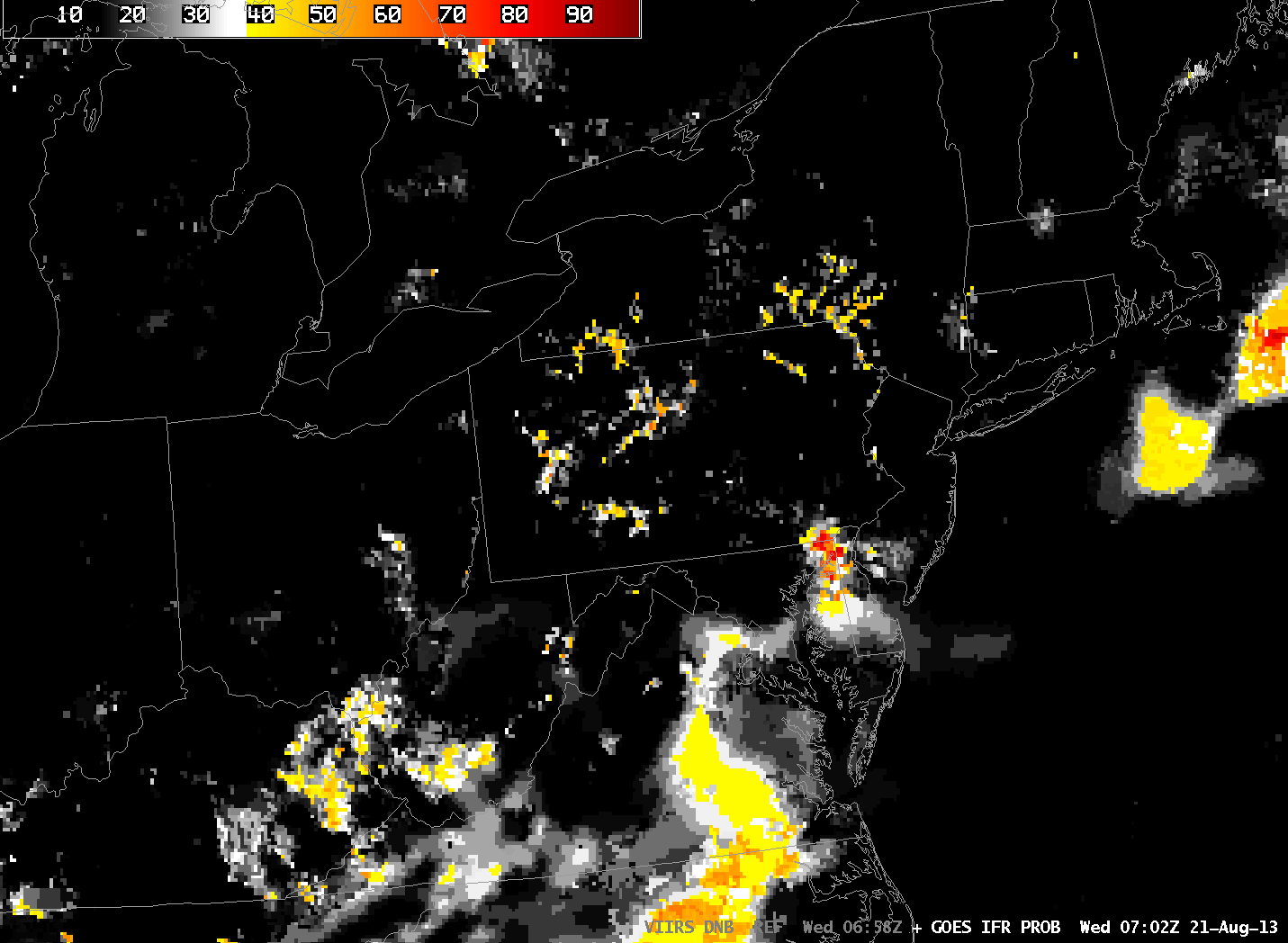
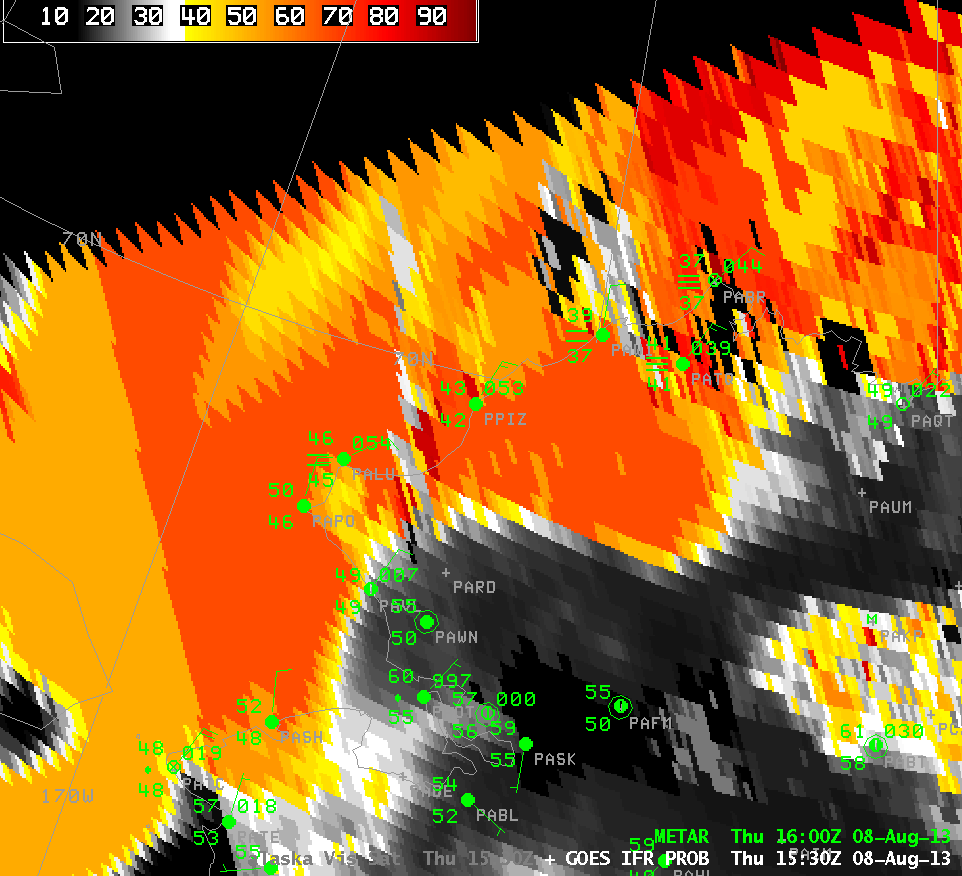
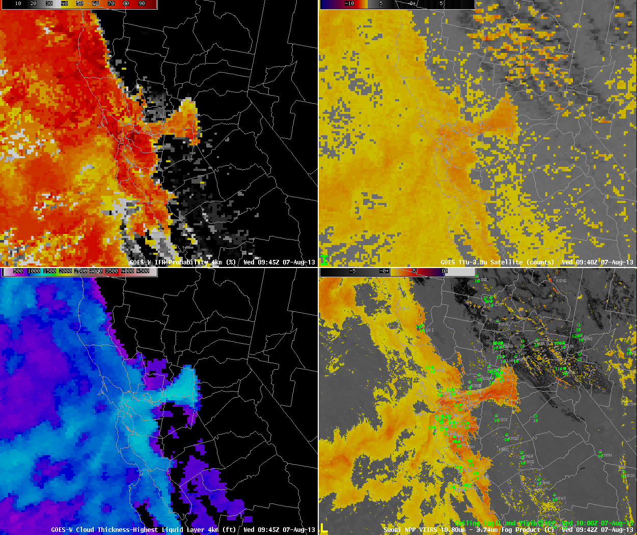
, GOES-West Brightness Temperature Difference (Upper Right, 10.7 µm - 3.9 µm), GOES-R Cloud Thickness (Lower Left), Suomi/NPP Brightness Temperature Difference (click image to play animation)

GOES-based GOES-R IFR Probabilities (Upper Left), GOES-West Brightness Temperature Difference (Upper Right, 10.7 µm – 3.9 µm), GOES-R Cloud Thickness (Lower Left), Suomi/NPP Brightness Temperature Difference (click image to play animation)

GOES-based IFR Probabilities track the incursion of a deck of marine stratus into metropolitan Sacramento and its surroundings on the morning of August 7. The cloud movement is also captured in the GOES-West (GOES-15) Brightness Temperature Difference fields. Note, however, how the GOES-R IFR Probability fields correctly suppress the signal in regions surrounding the stratus deck. These are regions where emissivity differences at 10.7 and 3.9 µm are more likely due to soil variability than to the presence of small liquid clouds droplets.

Suomi/NPP overflew the region at approximately 0945 UTC. The brightness temperature difference field for that time is shown here. The sharp edges of the stratus deck are readily apparent.

Although IFR Probabilities are high in this cloud bank, widespread IFR conditions were not reported. Much of the stratus was apparently elevated off the ground.

Some forecast models ably captured the evolution of this cloud field. A brightness temperature difference field from the 0000 UTC 7 August NSSL WRF, shown here (Courtesy of Dan Lindsey, NOAA) shows a cloud field evolving between 0900 and 1900 UTC on 7 August. Combining the forecast model output with real-time IFR Probability observations allows anticipation and monitoring of an evolving stratus deck.

Fog detection in the Upper Midwest

GOES-based GOES-R IFR Probabilities (Upper Left)
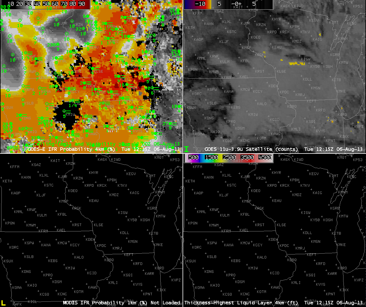
, GOES-East Brightness Temperature Difference (Upper Right, 10.7 µm - 3.9 µm), MODIS-based GOES-R IFR Probabilities (Lower Left), GOES-based GOES-R Cloud Thickness (Lower Right) (click image to play animation)

GOES-based GOES-R IFR Probabilities (Upper Left), GOES-East Brightness Temperature Difference (Upper Right, 10.7 µm – 3.9 µm), MODIS-based GOES-R IFR Probabilities (Lower Left), GOES-based GOES-R Cloud Thickness (Lower Right) (click image to play animation)

As nights lengthen in the upper Midwest in late Summer, the probability of fog development increases, especially on nights after light rainfall. The hourly animation, above, shows the gradual areal increase in high IFR probabilities that occurs as surface visibilities fall. Several aspects to the animation bear investigation. Note, for example, that at the start of the animation, the brightness temperature difference field, the traditional method used for fog detection, has a strong signal over eastern Illinois and western Indiana, a region where IFR conditions are not reported. This is a region of stratus clouds. Rapid Refresh model data that are incorporated into the GOES-R algorithm screens out these mid-level clouds; IFR probabilities in that region are correctly negligible. The end of the animation, 1215 UTC, occurs after sunrise, and reflected 3.9 µm solar radiation is affecting the brightness temperature difference field. The solar radiation complicates the use of the brightness temperature difference field as the sun rises. (Note also in that 1215 UTC image that GOES-R Cloud Thickness is not computed as it is during twilight conditions).

VIIRS_20130806toggle

The VIIRS instrument on board Suomi/NPP includes a day/night band that uses reflected Earth Glow and reflected lunar light to detect clouds. When the moon has set (or near times of the new moon — and the new moon occurs on August 6th, the date of these images), the scant illumination from Earthglow only makes low cloud detection a challenge. The brightness temperature difference product will still detect water-based cloudiness, however, as shown in the toggle above. However, the brightness temperature difference product does not include information on the cloud base, only on the cloud top. Incorporation of Suomi/NPP data into the GOES-R IFR Probability algorithm is ongoing.