Category Archives: Error Explanations

IFR Conditions over Maine

GOES-R IFR Probability and with surface observations of ceilings and visibilities, 1045 UTC on 13 February 2017 (Click to enlarge)

A strong storm off the East Coast of the United States produced a variety of winter weather over Maine on 13 February 2017, including Blizzard conditions. Although ceilings and visibilities above show IFR or near-IFR conditions at 1045 UTC, GOES-R IFR probabilities over Maine are small (less than 20%). Why?

The image below from this site shows Cloud Type, Low-Level Saturation, IFR Probability, and the Nighttime Microphysics.  Both Ice clouds and falling snow are widespread over Maine. GOES-R IFR Probabilities typically assume saturation with respect to water.   The Gray, ME morning sounding shows maximum RH (with respect to water) at only 94% (Link).  Assuming saturation with respect to water rather than with respect to ice may be a source of error that will have to be investigated in the future.

Note that after sunrise, IFR Probabilities increased over Maine to values between 30 and 45% (Link).

Satellite-derived Cloud Type (upper left), Maximum Low-Level Relative Humidity in the Rapid Refresh (upper right), GOES-R IFR Probability (lower left) and Nighttime microphysics (lower right), all from 1045 UTC on 13 February (Click to enlarge)

Power Outages

Two power outages 12 hours apart at UW-Madison CIMSS have impacted distribution of GOES-R IFR Probability fields. It’s possible that products may not be smoothly flowing again until Monday 13 June. Data are flowing as of about 0000 UTC on Saturday.

In the interim, users can find the products at the GEOCAT site. If you’re in the southeast US, near Atlanta, an experimental site that compares IFR Probability and Brightness Temperature Difference fields is here.

Occasional glitches in GOES-R IFR Probability fields from GOES-West

GOES_R_IFR_GOESW_0715to0745_27July2015anim

GOES-R IFR Probability fields computed using GOES-15 are periodically — once or twice per night — showing unusual behavior, as documented in the short animation above. The 0730 UTC shows a greatly expanded region of modest IFR Probability values compared to 0715 UTC; at 0745 UTC, fields return to ‘normal’. This aberrant behavior does not occur during the day, nor does it occur every night, nor at specific times. This intermittent type of error makes it difficult to determine and exact cause, but it appears to be related to GOES-15 3.9 µm emissivity. That field is missing when the erroneous fields are produced. This could be an issue of timing — that is, the algorithm requests the field before it is created.

CIMSS scientists are actively working to determine the underlying cause of this error.


======================== Added August 4 2015 =======================

Tweaks to the processing flow at CIMSS at the end of July appear to have fixed this problem, as it has not occurred in August.

Parallel Lines in IFR Probability over the Great Plains

GOES_IFR_PROB_20150612_1430

GOES-R IFR Probabilities over the Great Plains. Notice the north-south lines/artifacts in the field over Kansas and Nebraska (Click to enlarge)

GOES-R IFR Probability fields over the Plains can sometimes include structures as shown above. These are related to the sloped topography of the Great Plains. They occur because of interpolation between model layers and the lowest 1000 feet that are examined for saturation. In a sloping region, quick changes in saturation amount can occur where changing topography changes which model levels are used in the examination of those lowest 1000 feet.

In other words, satellite pixels that are very close horizontally may nevertheless have different surface elevations that cause different profile levels to be analyzed for the maximum relative humidity (RH). If the RH drastically changes at the bottom or top of the profile being analyzed then differences will emerge as shown above. Extra interpolation before the profile is analyzed may mitigate this issue and could be incorporated into the algorithm in the future.

When IFR Probabilities suddenly vanish

GOESIFR_PROB_Sunrise_11March2015

GOES-R IFR Probabilities over Indiana around sunrise on March 11 demonstrated what can happen when the Cloud Mask does not detect clouds, for whatever reason. The three-image loop above shows GOES-R IFR Probability at 1230, 1315 and 1330 UTC on 11 March. In the 1230 UTC image, the boundary between daytime predictors (to the east) and nighttime predictors (to the west) is manifest as a nearly north-south line through Kentucky and eastern Indiana. At 1315 UTC, a different boundary has appeared central lower Michigan, and this boundary moves westward to central Illinois at 1330 UTC. IFR Probabilities drop quickly to ~2% as this boundary passes, even though widespread IFR conditions are apparent. What is going on?

In this case, the cloud mask algorithm has failed to identify clouds over Indiana where clouds are present. A lack of clouds suggests Fog cannot be present. During the night, cloud masking is assigned less weight (because cloud detection is more difficult at night) so the cloud mask has a smaller impact on the IFR Probability. As night transitions into day, however, cloud masking acquires more importance in the computation of IFR Probability so the lack of a cloud will greatly influence IFR Probabilities. The IFR Probability algorithm also has a temporal check, so the effect of no cloud — as determined by the cloud mask — does not happen immediately as the sun rises. The animation below of cloud type shows no cloud type detected (starting at 1215 UTC over Michigan) in the regions where IFR Probabilities dropped. (That is, the cloud mask says no cloud is present; note also how IFR Probabilities do persist with the supercooled clouds over lower Lake Michigan, and with the clouds over southern Illinois).  Notice also how the cloud type returns over southern Illinois at 1315 UTC — the cloud mask is more accurate at that point.  Cloud masking identifies clouds over most of Indiana and Illinois by 1400 UTC; this can be deduced by the presence of cloud type values there.  The 1400 UTC GOES-R IFR Probability field, at bottom, shows IFR Probabilities redeveloping over Indiana and Illinois.

The Cloud Mask that is used by GOES-R IFR Probabilities is scheduled to be replaced with a more accurate (and more up-to-date) Bayesian Cloud Mask in the near future. This change, and GOES-R data (GOES-R is scheduled to launch on March 11 2016, in one year) will likely mitigate such cloud-masking errors as occurred on March 11 2015.

geocat.GOES-EAST.2015070.104500.to.143000.WISC.ctypeloop

GOES-13 Cloud Type, 1045 – 1430 UTC on 11 March 2015 (Click to enlarge)

GOES_IFRPROB_1400UTC_11March2015

GOES-R IFR Probabilities, 1400 UTC 11 March 2015 (Click to enlarge)

GOES-R IFR Probabilities at High Latitudes

MODIS_GOES_IFR_1300_27Oct2014

GOES-R IFR Probabilities computed using GOES-15 and Aqua Data, both near 1300 UTC on 27 October 2014 (Click to enlarge)

GOES-R IFR Probabilities are created using both GOES-15 Imager and Terra/Aqua MODIS. The toggle above shows MODIS-based IFR Probabilities (computed using data from Aqua and the Rapid Refresh) and GOES-based IFR Probabilities (computed using data from GOES-15 and the Rapid Refresh). There are three regions in the fields that warrant comment.

(1) Over East-central Alaska and the Yukon, large values of MODIS-based IFR Probabilities are limited in area (and near stations — such as Northway Airport — that are reporting IFR or near-IFR conditions). GOES-based IFR Probabilities in that same region include a large area with modest values — around 50%. Limb brightening may have an effect at high latitudes on the brightness temperature difference fields that are used in the computation of IFR probabilities because limb brightening is a function of wavelength. MODIS data (which will have far less limb brightening) can be used as a good check on the IFR Probabilty fields computed from GOES.

(2) Over Southwestern Alaska, and into the eastern Aleutians, GOES-based and MODIS-based IFR Probabilities are very similar. In this region, multiple cloud layers prevent satellite data from being used as a predictor in the computation of GOES-R IFR Probabilities. Rapid Refresh data is the main predictor for low clouds/fog, so MODIS-based and GOES-based fields will look similar.

(3) In the northeastern part of the domain, over the Northwest Territories of Canada, MODIS-based and GOES-based IFR Probabilities are very high. Satellite data are being used as a predictor here, and the satellite-based signal is strong enough to overwhelm any limb-brightening. (Note that southern Northwest Territories and northern British Columbia are south of the MODIS scan).

Terra- and Aqua-based MODIS observations yield frequent observations that result in good spatial and temporal coverage for IFR Probability fields over Alaska. GOES-15 temporal coverage is better, but the frequent MODIS passes can be used to benchmark GOES-based IFR Probability fields that may be misrepresentative because of limb-brightening effects at high latitudes.

Cloud Thickness as a Predictor of Fog Dissipation

GOES_R_Cloud_Thickness_1137UTC_18Sep2014

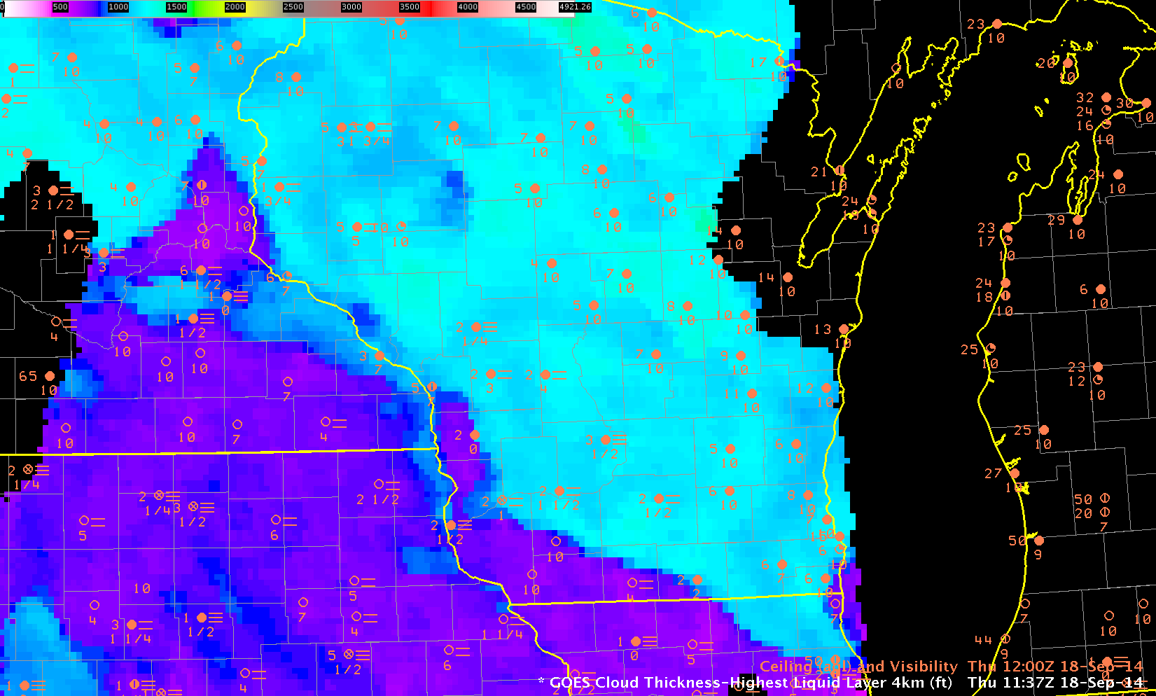
GOES-R Cloud Thickness over Wisconsin and surrounding States, 18 September 2014, just before sunrise (Click to enlarge)

GOES-R Cloud Thickness can be used as a predictor for dissipation time of Radiation Fog, using this chart and the thickness (as above) from the last pre-dawn GOES-R Cloud Thickness field (Recall that GOES-R Cloud Thickness is not computed in the few hours of twilight surrounding sunrise or sunset; in the image above, twilight has reached lower Michigan but not yet Wisconsin). However, it’s important to remember that the chart is valid for radiation fog. Other forcings might cause fog to dissipate (or persist).

In the example above, Cloud Thickness values ranges from around 700 over southwest Wisconsin to as much as 1400 over north-central Wisconsin. Most of south-central Wisconsin (cyan) has values around 1200. According to the best-fit line, that suggests a burn-off time of more than 5 hours (although those values are extrapolated; note that no values that large went into the creation of the best-fit line) over WI, except over southwestern WI where a burn-off time of less than 1 hour is predicted. Did that work out?

The animation below shows fog/low stratus moving towards the southwest with time. The cool and damp northeasterly flow from the Great Lakes into Wisconsin (surface map at 1800 UTC on 18 September) suppressed the heating necessary to reduce the relative humidity and foster fog evaporation. Perhaps the fog initially formed as advection fog; however, the northeasterly flow that developed early in the morning on 18 September came from a synoptic set-up that allowed fog to persist longer than the GOES-R Cloud Thickness algorithm suggests. This is not an uncommon occurrence. Clouds did not burn off over south-central WI until after 1800 UTC. During September, delayed burn-off of morning clouds can significantly affect the day-time temperature.

WIFOG_18Sep2014_12-20loop

Half-hourly visible imagery over Wisconsin, 1215-2045 UTC on 18 September (Click to animate)

=============================================================================

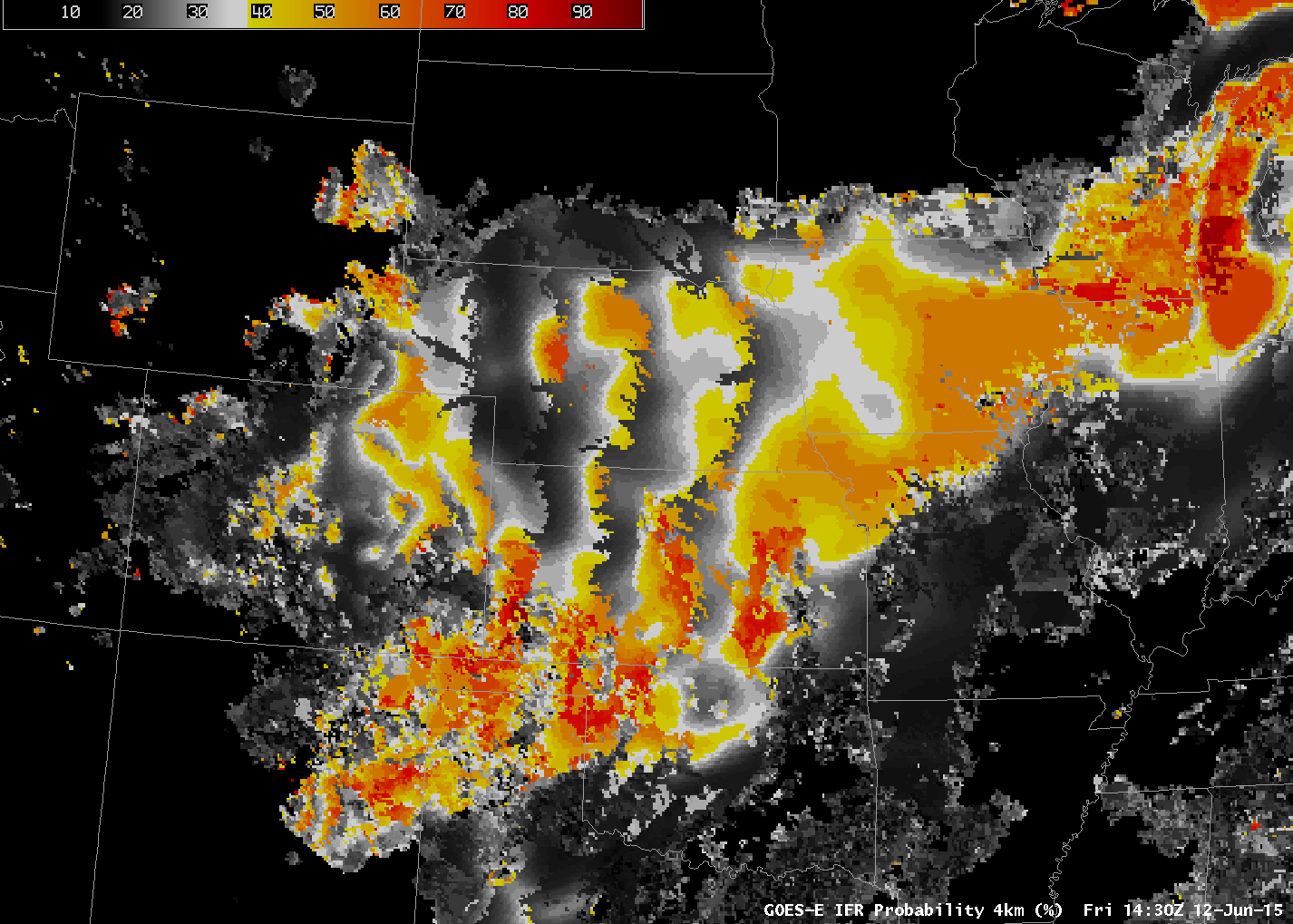
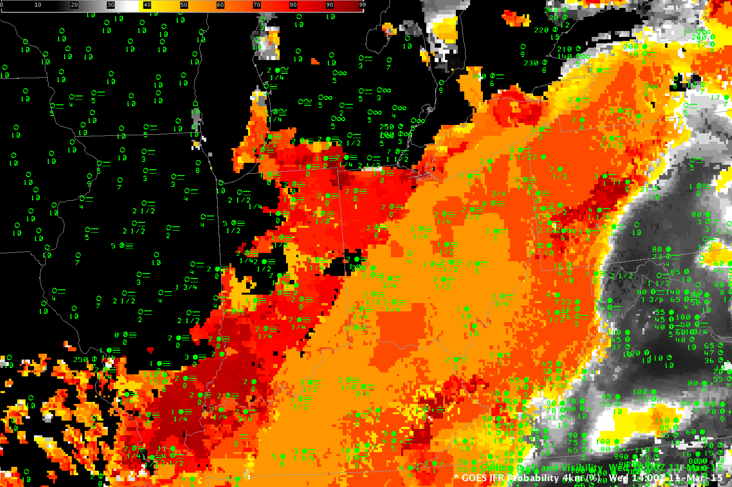
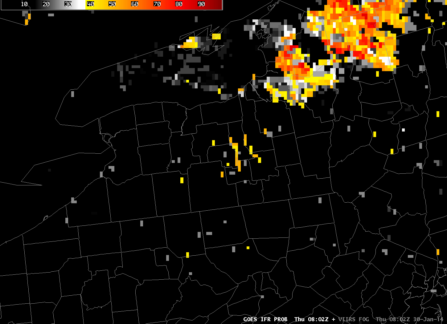
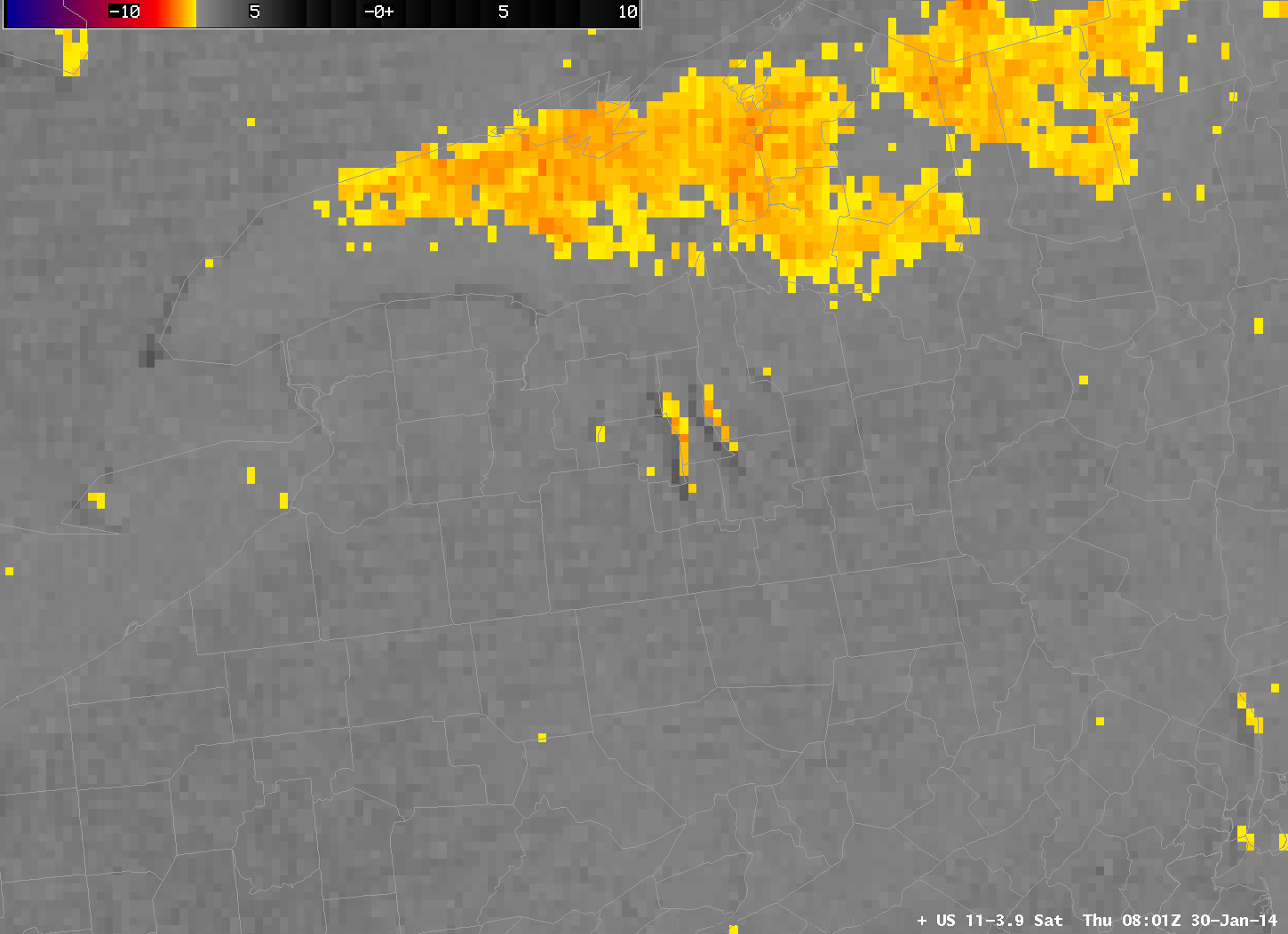
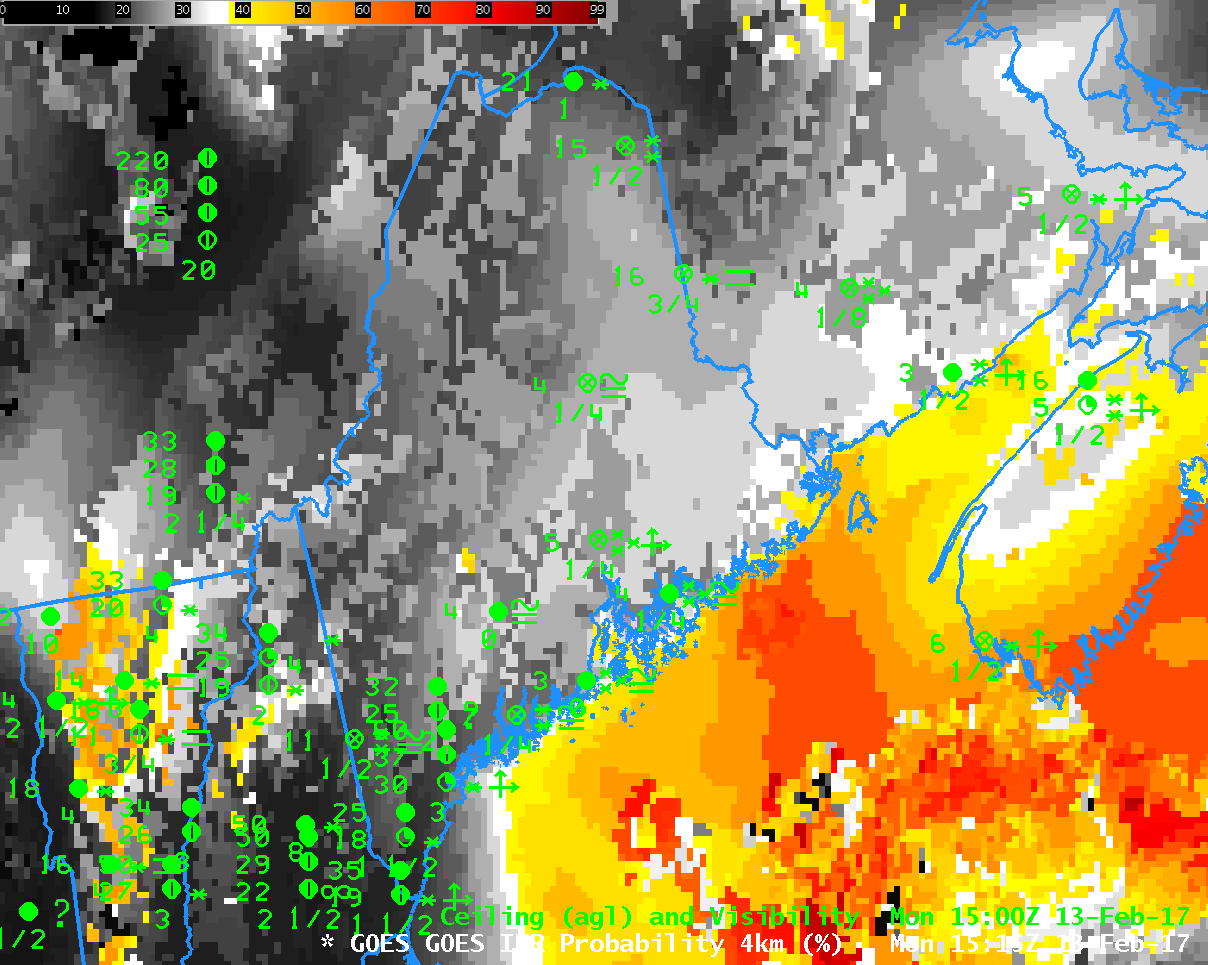
Low clouds and fog redeveloped during the morning of the 19th of September as well. This occurred during persistent southerly flow in advance of a low pressure system over the Northern Plains. The hourly animation of IFR Probabilities, below, shows IFR Probabilities developing over the course of the early morning of the 19th between 0315 and 1215 UTC. The animation shows a gradual overspreading of the IFR Probability field with higher clouds moving in from the west. (Here is a toggle between IFR Probability and GOES-13 Brightness Temperature Difference Fields at 1115 UTC; note how smooth the field is over much of WI where only Rapid Refresh model data can be used in the computation of the IFR Probability).

GOESR_IFRPROB_WI_19Sep2014_03-12

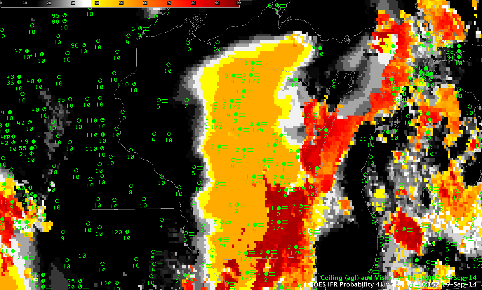
GOES-R IFR Probability fields, hourly from 0315-1215 UTC on 19 September (Click to animate)

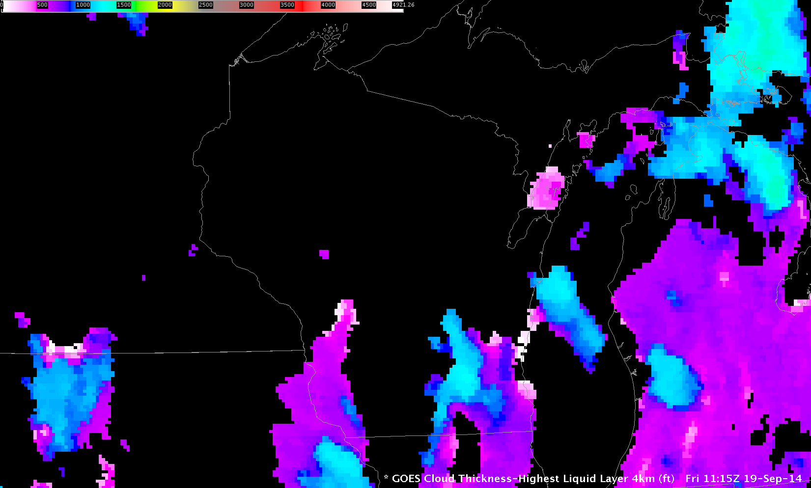
When high clouds overspread the scene, GOES-R Cloud Thickness is not computed. Thus, the last image before twilight, below, shows Cloud Thickness in only a few locations, but those values over southeast Wisconsin exceed 1200 feet, suggesting a burn-off of around 1615 UTC — 5 hours after this last Cloud Thickness image. In this case, that is an overestimate because the southerly winds over WI promote mixing, and the fog quickly dissipates after sunrise. It’s important to consider the synoptic forcing when you use Cloud Thickness. The last Cloud Thickness field and its use as a predictor for fog dissipation (using this chart) is most useful for radiation fog. The visible imagery animation at the bottom shows that the fog dissipated by 1415 UTC.

GOESR_CTH_WI_19Sept2014-9

GOES-R Cloud Thickness just before Sunrise (1115 UTC on 19 September 2015) (Click to enlarge)

WIFOG_19Sep2014_12-16loop

GOES-13 Visible Imagery, 1215-1615 UTC on 19 September (Click to animate)

GOES-R IFR Probability signal because of co-registration errors

GOES_IFR_PROB_20140130_0802

GOES-R IFR Probabilities at 0802 UTC, 30 January 2014 (click image to enlarge)

Special Update, 17 November 2014.

GOES-R IFR Probabilities on the morning of 30 January suggested the likelihood of fog along some of the Finger Lakes of upstate New York. These high probabilities arise because the Brightness Temperature Difference (10.7 µm – 3.9 µm) Product, below, shows a signal there. Note, however, that the Brightness Temperature Difference has a shadow; this is the sign that the co-registration error that is present between the 10.7 µm and 3.9 µm channels is producing a fictitious signal of fog over the lake. Such errors have been discussed here and elsewhere in the past.

US_11-3.9_Sat_20140130_0801

GOES-East Brightness Temperature Difference (10.7 µm – 3.9 µm) at 0801 UTC, 30 January 2014 (click image to enlarge)

Evidence that fog is not present is available in Suomi/NPP data taken at the same time as the GOES data, above. The toggle, below, of Day/Night Band imagery and of the brightness temperature difference (11.35 µm – 3.74 µm) from VIIRS shows scant evidence of fog/low stratus near the Finger Lakes. Because the moon is new, lunar illumination is at a minimum and surface features in the Day/Night band are not distinct, but the dark waters of the lakes are apparent.

VIIRS_FOGDNB_20140130_0802

Suomi/NPP VIIRS Day/Night band and Brightness Temperature Difference (11.35 µm – 3.74 µm) at 0802 UTC, 30 January 2014 (click image to enlarge)

MODIS data also suggests no fog/low stratus in the region. Both the brightness temperature difference field and the MODIS-based IFR Probabilities, below, support a forecast that does not mention fog around the Finger Lakes.

MODIS_FOG_IFRPROB_20140130_0746

MODIS Brightness Temperature Difference (11 µm – 3.74 µm) and MODIS-based GOES-R IFR Probabilities at 0746 UTC, 30 January 2014 (click image to enlarge)


=====================================================================

Update, 17 November 2014

NOAA/NESDIS has tested a software fix to align better the longwave infrared (10.7 µm) and shortwave infrared (3.9 µm) channels. The toggle below is of the Brightness Temperature Difference Field with (After co-registration correction) and without (Prior to co-registration correction) the realignment.

BTD_BeforeAfterFix

GOES-13 Brightness Temperature Difference Fields at 0802 UTC, 30 January 2014, with and without the co-registration correction as indicated (Photo Credit: UW-Madison CIMSS; Click to enlarge)

The correction of the co-registration error translates into more realistic IFR Probabilities in/around the Finger Lakes. In this case, IFR Probabilities are reduced because the false strong signal from the satellite is not present because of more accurate co-registration.

IFR_BeforeAfterFix

GOES-R IFR Probability fields computed Prior to and After co-registration correction, data from 0802 UTC 30 January 2014. IFR Probability fields with the corrected co-registration data are more accurate. (Photo Credit: UW-Madison CIMSS; Click to enlarge)

One more example of extreme cold

BTDIFR_20140127_1102toggle

Toggle of GOES-East Brightness Temperature Difference (10.7 µm – 3.9 µm) and GOES-R IFR Probabilities at 1100 UTC, 27 January 2014 (click image to enlarge)

One more example, above, showing the effects of extreme cold on the IFR Probability. IFR Probabilities correctly ignore the regions of low stratus in advance of the extreme cold air over Kansas and over the Ohio River Valley and Great Lakes. However, because of how the pseudo-emissivity is computed (See here also), and because the Rapid Refresh model show saturation in lower levels, regions with extreme cold will show a pixelated signal with noise.

IFR Probabilities in Extreme cold, Continued

GOES_IFR_Reg_11-3.9_Sat_20140106_0231loop


Toggle between GOES-R IFR Probabilities from GOES-13 and GOES-13 Brightness Temperature Difference (10.7 µm – 3.9 µm), with surface observations and ceilings plotted, ~0230 UTC on 6 January 2014. (click image to animate)

The coldest air of the season has plunged into the central part of the US. And as noted before, extreme cold does have an influence on the IFR Probability fields because of how the pseudo-emissivity is computed. Consider this effect of cold on the fields as you interpret them. Note also that in the daytime, when visible imagery can be used to augment the cloud mask, IFR Probabilities are low in very cold airmasses.