GOES-16 ‘Fog Detection’ Channel Difference (10.3 µm – 3.9 µm), 0912 – 1132 UTC, 29 June 2017 (Click to enlarge)

GOES-16 data posted on this page are (still!) preliminary, non-operational data and are undergoing testing

The 16 channels on the GOES-R Series Advanced Baseline Imager (ABI) allow for many different channel combinations that can be used to detect atmospheric phenomena. The animation above shows the traditional method for detecting low stratus: the brightness temperature difference between the shortwave infrared (3.9 µm) and the cleanest longwave infrared (10.3 µm) windows. Cloudtops composed of water droplets are highlighted in the animation because they do not emit 3.9 µm radiation as a blackbody, but do emit 10.3 µm radiation as a blackbody; thus, the brightness temperature difference at night (when no reflected solar radiation at 3.9 µm is present) is positive. The range of the colorbar in the above animation is from -50 to +50 C; stratus appears as green over much of northern Wisconsin, Minnesota and North Dakota.  Higher cirrus clouds are cyan, and they interfere with the satellite detection of low clouds, especially over eastern North Dakota where IFR conditions were widespread (source), and where a Dense Fog Advisory existed.  Note the apparent disappearance of the fog signal — in green — as the sun rises.  Increasing amounts of reflected solar radiation are causing the brightness temperature difference value to switch sign from (10.3 µm – 3.9 µm) > 0 at night (because of emissivity differences) to (10.3 µm – 3.9 µm) < 0 during the day (because of solar reflectance).

The ‘Nighttime Microphysics Advanced RGB’ is also used as a fog detection device. In the animation below, low stratus (and by inference, fog) is highlighted in cyan, a signal that comes mostly from the ‘green’ part of the RGB, namely the Brightness Temperature Difference as shown above. Because the two products are linked by the 10.3 – 3.9 brightness temperature difference, shortcomings in that product as far as fog detection affect the RGB. Note how the fog signal erodes over Minnesota/Wisconsin as the sun rises, and how it is obscured by high clouds (dark purple/magenta) over North Dakota.

Note: GOES-R IFR Probabilities are computed using Legacy GOES (GOES-13 and GOES-15) and Rapid Refresh model information; GOES-16 data will be incorporated into the IFR Probability algorithm in late 2017

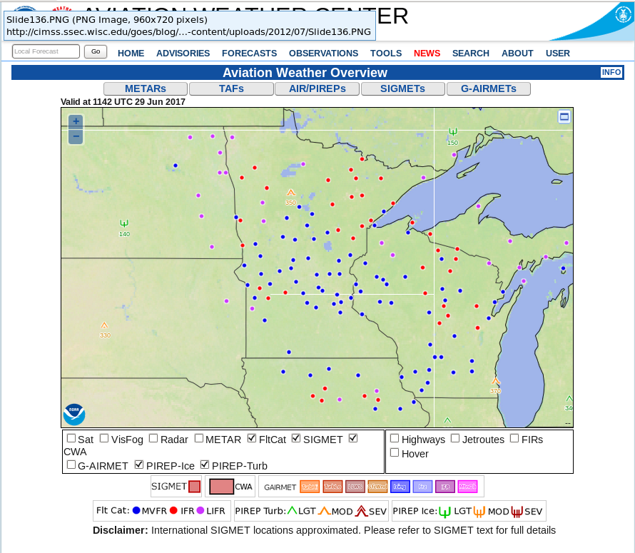
GOES-R IFR Probability fields, shown for this event below, were designed to mitigate detection issues noted above.  Where high clouds are present, meaning the satellite cannot detect low clouds, information about low-level saturation from the Rapid Refresh is used to assess whether or not fog is likely.    That low-level information from the model also can be used to distinguish between fog and elevated stratus that can look very similar from the top, as a satellite views it.  The fusing of model and satellite data makes for a product that has better statistics in detecting low ceilings and reduced visibilities.

At the end of the two animations above, for example, how confident will a satellite analyst or forecaster be that there is dense fog over eastern North Dakota?  How about the analyst/forecaster using IFR Probability fields? IFR Probabilities maintain a signal for fog over the entire region from North Dakota to Wisconsin, even through sunrise and under high clouds.

GOES-R IFR Probabilities, 0915 to 1115 UTC on 29 June 2017 (Click to enlarge)