Monthly Archives: September 2015

Fog/Low Stratus over coastal Oregon

SNPP_DNB_30Sep2015_0944_1125animg

Suomi NPP Visible Imagery from the Day Night Band, 0944 and 1125 UTC on 30 September 2015 (Click to enlarge)

The near-Full Moon provided ample illumination of fog/low stratus near the Oregon Coast early in the morning of 30 September, as shown above. Note also the clear skies near North Bend along the southern Oregon coast. What did the GOES-R IFR Probability field show at these two times?  IFR Probability fields also suggest clear skies around North Bend/Coos Bay (and offshore), as observed.  The fine fingers of fog/low stratus that are moving up river valleys in the 1125 UTC image most notably are not resolved by GOES-15 (which has a 4-km pixel size at the sub-satellite point). Both fields do capture the slow increase in cloud cover over land. Available surface observations show near-IFR conditions at some stations in Oregon.

GOES15_IFRPROB_30Sep2015_0944_1115anim

GOES-R IFR Probabilities computed with GOES-15 and Rapid Refresh Data, 0945 and 1115 UTC on 30 September 2015 (Click to enlarge)

IFR Probabilities give information during the day too

IFRPROB_24Sep2015_13-17anim

GOES-R IFR Probabilities, hourly from 1300-1700 UTC on 24 September 2015 (Click to enlarge)

Ceilings and visibilities over South Carolina decreased during the day on 24 September 2015. The animation of hourly IFR Probability fields, above, shows an increase in Probability over South Carolina as the visibilities decreased.  IFR Probability fields can alert a forecaster to the possibility of IFR conditions at any time of the day.   Visible imagery for the same period, below, shows the multiple cloud layers streaming inland. The accuracy of the IFR Probability field in highlighting the region with near-IFR and IFR Probability is testimony to the accuracy of the Rapid Refresh model data that are used.

VIS_1300_1700_24sept2015anim

GOES-East Visible (0.63 µm) Imagery, hourly from 1300-1700 UTC on 24 September 2015 (Click to enlarge)

IFR Probability vs. Brightness Temperature Difference

GOES_IFR_BTD_1000_21Sept2015toggle

GOES-R IFR Probability and GOES-13 Brightness Temperature Difference (10.7 µm – 3.9 µm) at 1000 UTC on 21 September 2015 (Click to enlarge)

The toggle above compares GOES-R IFR Probability fields and GOES-13 Brightness Temperature Difference fields at 1000 UTC on 21 September 2015. A shortcoming of Brightness Temperature Difference fields, or indeed of any low cloud detection algorithm that relies solely on cloud-top measurements, is that low stratus that does not reduce visibility and fog that does reduce visibility can look very similar from the cloud top. By incorporating surface and near-surface moisture information from the Rapid Refresh Model, the GOES-R IFR Probability algorithm can correctly screen out regions of stratus and highlight only those regions where fog and low stratus might affect transporation. In the example above, Guymon OK and Lamar CO are at the outer edge of the highest IFR Probability, and both report IFR conditions. South and west of those stations, IFR Probabilities drop quickly, but brightness temperature difference signals remain strong.

Cloud Thickness and Dissipation Time

Slide136

Dissipation time as a function of GOES-R Cloud Thickness

The chart above shows the relationship between the last pre-sunrise GOES-R Cloud Thickness product and Fog Dissipation time.  Observations of the last pre-sunrise GOES-R Cloud Thickness (developed from an empirical relationship between 3.9 µm emissivity and sodar-observed cloud thickness of the west coast of the USA) can be related to the dissipation time relative to the last observation of Cloud Thickness.  The scatterplot was developed using data mostly over the southeastern part of the USA, but also over the Great Plains.  However, it does have value in other geographic regions too, as shown below.

GOESR_CLDTHICK_IFRPROB_1100UTC_16sep2015toggle

GOES-R IFR Probabilities and GOES-R Cloud Thickness, 1100 UTC 16 September 2015 (Click to enlarge)

On 16 September, river fog developed over the Ohio River and its tributaries in Ohio, West Virginia and Pennsylvania. The toggle above shows GOES-R IFR Probability and GOES-R Cloud Thickness fields at 1100 UTC on 16 September.  This was the last pre-sunrise GOES-R Cloud Thickness over West Virginia (Indeed, the leading edge of twilight — where GOES-R Cloud Thickness is not computed — is apparent at the extreme eastern edge of the image, from Virginia up into central Pennsylvania). The GOES-R Cloud Thickness fields show largest values — around 800 feet — in/around the Ohio River between West Virginia and Ohio. The chart above suggest rapid dissipation. The best fit line (blue) suggests dissipation in about an hour, although there is considerable spread to the values, from 30 minutes up to almost 2-1/2 hours.

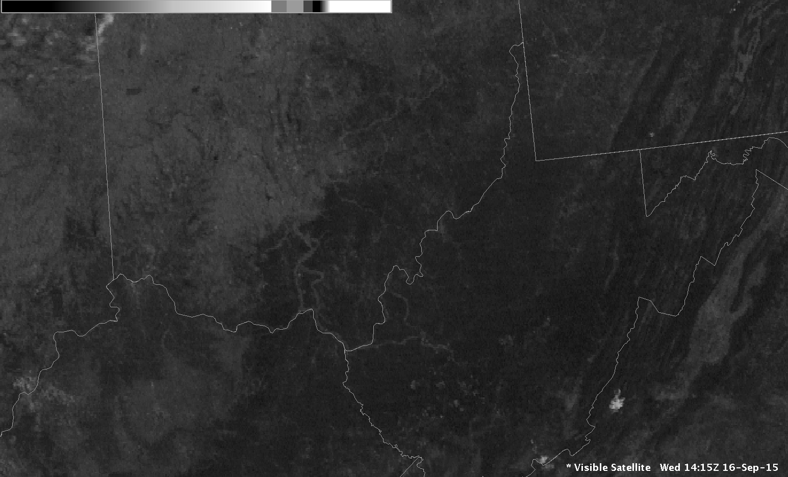
Almost two hours later (1245 UTC), fog is still present in isolated patches near the river, and GOES-R IFR Probability fields are suggesting fog is still present as well.  The horizontal extent of the GOES-R IFR Probability field is greatly reduced because visible imagery can be used after sunrise to screen out clear regions (Cloud-clearing in the algorithm is more effective).  By 1415 UTC (bottom), three hours after the GOES-R Cloud Thickness imagery above, all fog has evaporated.

GOES_VIS_GOESRIFRPROB_1245UTC_16sep2015toggle

GOES-R IFR Probabilities and GOES-13 Visible Imagery (with a low-light enhancement), 1245 UTC 16 September 2015 (Click to enlarge)

GOES_VIS_1415UTC_16sep2015

GOES-13 Visible Imagery, 1415 UTC 16 September 2015 (Click to enlarge)

MODIS resolution versus GOES resolution

WV_MODIS_GOES_IFRPROB_0315_11Sep2015toggle

MODIS-based (0300 UTC) and GOES-based (0315) UTC GOES-R IFR Probability fields on 11 September 2015 (Click to enlarge)

MODIS data (from Terra and Aqua) and GOES data can both be used to create GOES-R IFR Probability fields. The differences between the two data sources — especially spatial resolution — are obvious in the toggle above. MODIS data can capture the development of fingers of fog that develop in small river valleys, and GOES data cannot (although, of course, a forecaster with knowledge of the topography might appropriately tailor a forecast). In the toggle above, MODIS data capture the small tributaries of the Ohio River in Ohio and West Virginia that likely contain fog at 0300 UTC (11 PM local time). GOES data smear out that information. This is true later at night as well, below, at 0715 UTC. River valleys show higher IFR Probabilities than adjacent mountains. Valley fog is easier to delineate with MODIS data than with GOES data.

WV_MODIS_GOES_IFRPROB_0715_11Sep2015toggle

MODIS-based (0715 UTC) and GOES-based (0715) UTC GOES-R IFR Probability fields on 11 September 2015 (Click to enlarge)

GOES-R IFR Probabilities at High Latitudes

AK_DenseFog_8Sep2015

Screenshot from the Juneau, AK WFO on 8 September 2015. The yellow region has a Dense Fog Advisory (Click to enlarge)

A challenge in using GOES-R IFR Probabilities at high latitudes is that GOES pixels are larger, typically twice or three times the size of pixels over the lower 48. If Fog is starting out as a small-scale phenomenon, the early development of the feature can be missed. Dense fog developed over southeast Alaska on the morning of 8 September. The animation of GOES-15-based IFR Probabilities, below, shows the slow increase in areal extent to the IFR Probabilities in the six hours between 0445 and 1045 UTC; values also increased.  This slow increase in concert with observations can increase confidence that wide-spread dense fog is possible.

AK_GOES_IFRPROB_0445_1045UTC_08Sept2015stepanim

GOES-15 based GOES-R IFR Probabilities, 0445, 0715 and 1045 UTC on 8 September 2015 (Click to enlarge)

MODIS data from Terra and Aqua can also be used to compute IFR Probabilities, and the high resolution information from these two polar orbiting satellites can clarify where fog might be occurring. Additionally, MODIS fields are a bit more frequent over Alaska than they are over the lower 48. The 0600 and 0737 UTC passes, shown below, show how MODIS data can be used to refine the GOES-based information at times during the night. The temporal change between MODIS information at 0600 and 0737 UTC also confirms the trend observed in GOES data alone.

AK_GOES_MODIS_IFRPROB_0600UTC_08Sept2015toggle

GOES-15 and MODIS-based GOES-R IFR Probabilities, 0600 UTC 8 September 2015 (Click to enlarge)

AK_GOES_MODIS_IFRPROB_0730UTC_08Sept2015toggle

GOES-15 and MODIS-based GOES-R IFR Probabilities, ~0730 UTC 8 September 2015 (Click to enlarge)