Category Archives: Emissivity

IFR Conditions with a Spring storm over the central United States

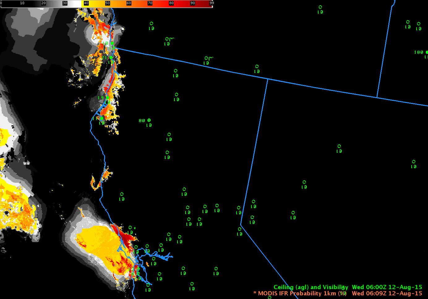
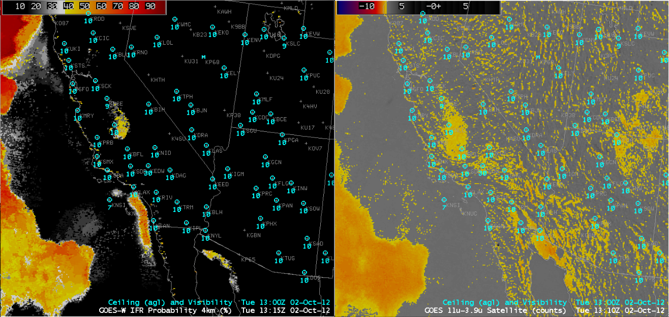
GOES-16 IFR Probability fields, every 10 minutes, from 0202 through 1412 UTC on 19 March 2018 (Click to animate)

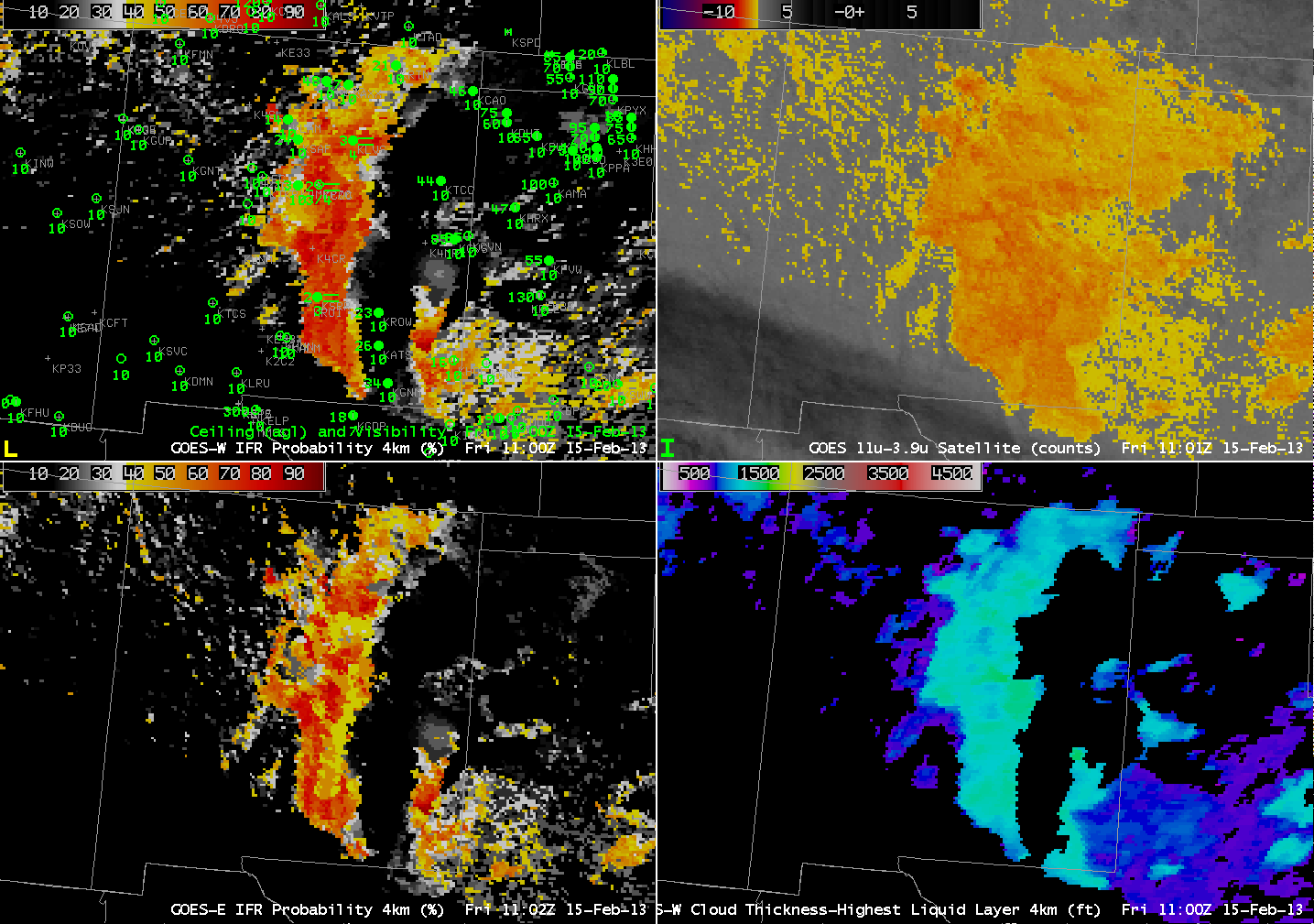
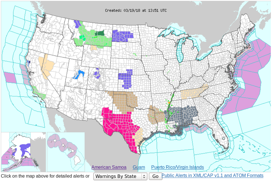
Dense Fog Advisories (click here for graphical image from this site) and widespread IFR Conditions (click here for graphical image from this site) occurred as a nearly-occluded system spun slowly eastward across the central part of the United States on 19 March 2018. (Surface; 500-hPa). GOES-16 IFR Probability, shown above, (Click the image to see the animation) outlines two large areas where consistent IFR conditions develop/persist: the upper Plains, in states around Nebraska, and the Deep South.

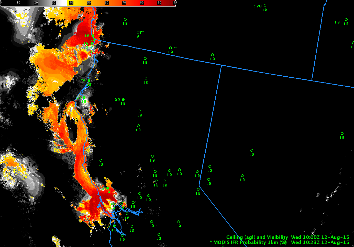
The GOES-16 Night Fog Brightness Temperature Difference field (10.3 µm – 3.9 µm), animation shown below, historically has been used to identify low stratus that is assumed to be fog at night. That detection suffers when high clouds are present (consistently on the morning of 19 March over Nebraska and surrounding states; occasionally over the Deep South as convection expels high-level cirrus into the atmosphere). Because IFR Probability fuses satellite data with Numerical Model estimates of low-level saturation (from the Rapid Refresh Model), it retains a strong signal of fog in regions where multiple clouds layers prevent the satellite from observing observed low stratus causing IFR conditions, such as over Nebraska, or over Mississippi at 0607 UTC.

GOES-16 Night Fog Brightness Temperature Difference (10.3 µm – 3.9 µm), 0202-1412 UTC on 19 March 2018 (Click to animate)

Note that there exists a Brightness Temperature Difference signal over the High Plains of Texas and New Mexico at, for example, 0800-0900 UTC. (See below). Persistent drought exists in that region (linked image from this site) and the dryness can alter the relative emissivities of the soils so that a signal develops (Click here for an earlier example).  There are no clouds in this region;  the Rapid Refresh model shows very dry air and the IFR Probability algorithm correctly diagnoses very small probabilities of IFR conditions.

GOES-16 Night Fog Brightness Temperature Difference (10.3 µm – 3.9 µm), 0802-0902 on 19 March 2018 (Click to enlarge)

Coastal California Fog

NPP_DNB_BTD_1003UTC_12August2015toggle

Toggle between Suomi NPP Day Night Band Visible (0.70 µm) Image and Brightness Temperature Difference (11.45 µm – 3.74 µm) , 1003 UTC 12 August 2015 (Click to enlarge)

Suomi NPP data from 1003 UTC on 12 August, above, shows evidence of a cloud bank hugging the northern California coast from Cape Mendocino to San Francisco Bay. It also penetrates inland to Santa Rosa in Sonoma County. (Note also how the fires burning in interior show up well in the Day Night Band — they are emitting visible light — and in the Brightness Temperature Difference band — because they are much warmer in the 3.74 µm image than in the 11.45 µm image).

Terra overflew the California coast at ~0600 UTC and Aqua overflew the coast at ~1000 UTC; MODIS-based IFR Probabilities could be constructed from these overpasses, and they are shown below.  At 0609 UTC, High IFR Probabilities (>90%) are confined to coastal Sonoma County and along the coast from Humboldt county north.  By 1023 UTC, high IFR Probabilities stretch along the entire coast from Cape Mendocino to the mouth of San Francisco Bay, with evidence of inland penetration along river valleys.  (The Russian River, for example, and perhaps the Noyo River in Mendocino County)

MODIS_IFR_0609UTC_12August2015

Terra MODIS-based GOES-R IFR Probability fields, 0609 UTC, 12 August 2015 (Click to enlarge)

MODIS_IFR_1023UTC_12August2015

Aqua MODIS-based GOES-R IFR Probability fields, 1023 UTC, 12 August 2015 (Click to enlarge)

MODIS can give high-resolution imagery, but the infrequency of the scenes tempers its usefulness. In contrast, GOES-15 (as GOES-West) views the California coast every 15 minutes, and this excellent temporal resolution (that will improve in the GOES-R era) allows a better monitoring of the evolution of coastal fog. Hourly plots of GOES-R IFR Probability, below, computed from GOES-15 and Rapid Refresh Data show the slow increase in GOES-R IFR Probabilities along the coast as ceilings and visibilities drop.

GOESWIFR_12August2015_0400_1200anim

GOES-R IFR Probability fields, 0400-1200 UTC 12 August 2015 (Click to enlarge)

In the animation above, note the general increase in GOES-R IFR probabilities at 0900 UTC relative to 0800 and 1000 UTC. We are close enough to the Solstice that Stray Light Issues are starting. The 0800, 0900 and 1000 UTC brightness temperature difference imagery, below, shows the large signal increase at 0900 UTC that can be attributed to stray light. GOES-R IFR Probabilities can tone down that increase somewhat — because the model data will now show low-level saturation in regions where stray light erroneously suggests low clouds/fog might exist. GOES-R IFR Probabilities also screen out the constant fog signal over the Central Valley of California (and over Nevada) that is driven not by the presence of low clouds but by soil emissivity differences.

GOESWBTD_12August2015_0800_0900_1000step

GOES-15 Brightness Temperature Difference (10.7 µm – 3.9 µm), 0800, 0900 and 1000 UTC 12 August 2015 (Click to enlarge)


======================== Added =========================
GOES-14 in SRSO-R mode (see also this link) viewed the west coast starting at 1115 UTC today. The Brightness Temperature Difference field, below, (click here for mp4) shows the slow expansion/evaporation of the low stratus/fog. (GOES-R IFR Probabilities were not computed with the GOES-14 1-minute imagery). The rapid change in the field at sunrise occurs because solar radiation at 3.9 µm quickly changes the brightness temperature difference from negative to positive.

Visible Imagery is below (Click here for mp4).

960x1280_AGOES14_B1_GOES14_W_animated_2015224_133000_182_2015224_170000_182_GRAY

GOES-14 Visible Imagery (1330-1700 UTC) (Click to animate)

Pseudo-emissivity at 3.9 µm

The traditional (or heritage) method of detecting fog/low clouds is a brightness temperature difference (BTD) product. The difference between brightness temperatures at 10.7 µm and 3.9 µm highlights water-based clouds because those clouds do not emit as a blackbody at 3.9 µm, so the inferred temperature (computed assuming a blackbody emission) is colder than that temperature computed using 10.7 µm radiation, because clouds emit radiation at 10.7 µm more like a blackbody.

At night, the GOES-R IFR Probabilities use a pseudo-emissivity at 3.9 µm in lieu of the 3.9-11µm BTD to highlight regions of water-based clouds at low levels. The 3.9 µm Pseudo-emissivity is the ratio of the observed radiance at 3.9 µm to a computed 3.9 µm blackbody radiance that is based on the observed 10.7 µm brightness temperature. In other words, the observed 10.7 µm brightness temperature is computed from the 10.7 µm radiance. That computed brightness temperature is then used to compute a 3.9 µm radiance that would be detected if the emitter was a blackbody.

The 3.9 µm pseudo-emissivity produces a satellite signature for low water clouds similar to the brightness temperature difference but is used instead because it is less sensitive to scene temperature. Skill scores for fog/low stratus detection are higher when the pseudo-emissivity is used in the algorithm to find regions of low clouds/fog than when the brightness temperature difference field is used.

GOES-13 outage

Half-hourly imagery of GOES-R IFR Probability (Upper Left) computed from GOES-West, GOES West Brightness Temperature Differences (10.7 – 3.9) (Upper Right), GOES-R Cloud Thickness (Lower Left), GOES-R IFR Probability from MODIS (Bottom right)

GOES-13 has experienced an anomaly, and is in safe mode.  While this occurs, GOES-15 will operates in full-disk mode.   GOES-R IFR Probability coverage is therefore limited east of the Missouri River Valley.  When GOES-14 starts transmitting imagery, starting at around 0500 UTC 23 May, GOES-East projections of GOES-R products will resume.  In the meantime, coverage along the East Coast is provided — at high resolution — by the MODIS-based GOES-R products, shown below. Temporal resolution is degraded in this polar-orbiter-based product, however.

The image loop above spans several MODIS IFR Probability products, but the MODIS products are not close enough to the half-hourly time steps to be included in the imagery.  The GOES-West-based IFR probability products identify the four main regions of reduced visibilities overnight:  the Pacific Northwest, southern California, the northern Plains, and east Texas.  Other regions that show a strong return in the brightness temperature difference product have either elevated stratus (Texas Panhandle) or soil with variable emissivity properties (the intermoutain West).

GOES-R IFR probabilities computed from MODIS data, 0230 UTC – 1000 UTC, 22 May 2013

GOES-R IFR Probabilities Refine the Area of IFR Conditions over New Mexico

GOES-R IFR Probabilities from GOES-West (Upper Left), GOES-R IFR Probabilities from GOES-East (Lower Left), GOES-East Brightness Temperature Difference (10.7 µm – 3.9 µm) (Upper Right), GOES-R Cloud Thickness of Highest Liquid Layer computed from GOES-West (Lower Right), all from 1100 UTC on 15 February 2015

Because GOES-R IFR Probabilities include information about the near-surface atmosphere in the Rapid Refresh Model (and therefore, through assimilation into that model of surface data, the actual atmosphere), IFR probabilities do a better job of distinguishing elevated stratus from fog/low stratus.  In the image above from 1100 UTC on 15 February, the GOES brightness temperature difference product, the traditional method of alerting forecasters to the possibility of fog, shows a signal over the high plains of eastern New Mexico in regions where observations show high ceilings. The GOES-R Fog/Low Stratus product computed from either GOES-West data (top left) or GOES-East data (bottom left) correctly restricts the possibilities of IFR conditions to regions between the Sangre de Cristo mountains in the north to the Sacramento mountains in the south.

Difficulties detecting FLS over arid regions using satellite alone.

GOES-R IFR probabilities (top left) and the traditional 3.9-11 micron brightness temperature difference (top right) from GOES-West on October 2, 2012 at 13:30 UTC. The blue circles are surface observations with the surface visibility (in miles) below. 
The maximum relative humidity in the lowest 1000ft layer above ground level from the Rapid Refresh forecast model valid at 13:15 UTC on October 2, 2012.
The traditional 3.9-11 micron brightness temperature difference (BTD) used to detect liquid stratus clouds exploits the emissivity differences at the 3.9 and 11 micron wavelengths. Liquid water clouds typically emit less at 3.9 microns than at 11 microns and this difference can be used to differentiate them from other types of clouds. This method works well when the liquid stratus clouds are the highest cloud layer and are distinguishable from the background surface characteristics. However, fog/low stratus (FLS) detection over arid regions can be difficult using satellite data alone because the very dry land surface typically has a low surface emissivity at the 3.9 micron wavelength as well, resulting in a satellite signal very similar to that of liquid stratus clouds. This is shown in the top right image above where the arid regions of the SW U.S. have a similar BTD signal as the status clouds offshore California even though all the surface observations in the area indicate no clouds are present. 
The GOES-R IFR product (top left image above) can greatly reduce the false satellite signal caused by the land surface by incorporating model relative humidity (RH) data. For the GOES-R IFR product the satellite data is combined with the maximum RH found in the lowest 1000 ft layer above ground level from the Rapid Refresh RH profiles using a naive bayesian probabilistic model. FLS generally occurs when the low-level RH is relatively high (> 80%). The low level RH in arid regions is usually very low (< 30%), so even when the satellite signal is strong, indicating FLS may be present,  the weak model signal works to lower the probability that FLS is present. 
However, sometimes the low-level RH can be elevated over dry land surfaces when clouds are not present. When this occurs, the relatively high model signal along with the relatively high satellite signal (from the land surface) indicate there is a greater chance that FLS may be present so the GOES-R IFR probabilities are slightly elevated. This is shown in the top left image above where an area of elevated GOES-R IFR probabilities in central California indicate that there is a roughly 40% chance that IFR conditions are present even though the surface stations report clear skies. The low-level modeled RH from the Rapid Refresh model (bottom image above) indicates a sliver of elevated RH (> 80%) in central California. This area of elevated low-level RH combined with the relatively higher satellite signal (from the land surface) resulted in the GOES-R IFR probabilities being slightly elevated. GOES-R IFR probabilities around 40% are considered to be relatively low and, combined with the surrounding surface observations, forecasters should feel pretty confident that this is indeed a false signal and that FLS is not present.

GOES-R IFR probabilities (left) and the traditional 11-3.9 micron brightness temperature difference (right) from MODIS on October 2, 2012 at 9:05 UTC. The blue circles are surface observations with the surface visibility (in miles) below.

The higher spatial resolution (1 km) MODIS instrument shows in more detail the elevated traditional BTD satellite signal caused by the arid land surface (right image) over the SW U.S. The GOES-R IFR probabilities applied to MODIS (left image) again show how the GOES-R IFR product significantly reduces the false FLS signal that is seen in the traditional BTD product.

Emissivity properties in a drought

GOES-R IFR Probabilities (upper left), Total Precipitable Water (the so-called ‘Blended Product’) (upper right), 10.7 µm – 3.9 µm Brightness Temperature Difference (lower left), Enhanced Water vapor imagery with surface observations (lower right)

The driving mechanism in the brightness temperature difference product, the heritage method for detecting fog and stratus from satellites, keys on differences in the emissivity of water clouds at 3.9 µm versus the emissivity at 10.7 µm.  Water clouds do not emit 3.9 µm radiation as a blackbody does, but they do emit 10.7 µm radiation almost as a blackbody.

As ground dries out in a drought, its emissivity changes. Those changes are a function of wavelength.  This example is from early morning on 31 August, as the remnants of Isaac slowly spread northward.  The brightness temperature difference shows a strong signal around the cirrus canopy of the storm.  These highlighted regions arcing from Kansas to Illinois have suffered extreme drought all summer.  The satellite signal is so strong in this case over the very dry Earth — because of the changed emissivity properties of the parched Earth — that it cannot be overcome by the model parameters that are used.  As a result, IFR probabilities are high over Indiana and Illinois where no IFR conditions are observed.