Day/Night Transition artifacts

GOES-R IFR Probability, 1430 UTC on 25 October 2012

The predictors used by the GOES-R IFR Probability algorithms change as night turns to day and vice versa.  For example, the daytime predictors include the visible satellite imagery.  The change in predictors occurs when the solar zenith angle is less than 85 degrees (that is, when the sun is just rising). For solar angles between 85-90 degrees, temporal continuity has an increased importance and therefore the IFR probabilities look very similar to the previous temporal images.  When the solar zenith angle is between 80-85 degrees temporal metrics are used combined with current visible channel data (only if certain tests are passed that prove the data is of good quality). The cloud mask sometimes has difficulty detecting low clouds in this region so it still is not fully utilized until the solar zenith angle drops to below 80 degrees, where the cloud mask and the full array of daytime predictors are used. This leads to discernible changes in the probability fields, as shown above.  Two boundaries, extending southwest to northeast (roughly parallel to the terminator) are apparent, one from extreme northwest Utah through central Montana and into Canada (where the solar angle is around 85 degrees) and one from northwest Colorado through northwest South Dakota into Manitoba (where the solar angle increases above 80 degrees).   This transition zone is less noticeable in the Summer because of the Earth-Sun geometry.  It is very difficult to create the GOES-R Cloud Thickness product when the solar zenith angles are between 75-90 degrees so the product is currently not available in this region.  This is why the Cloud Thicknesses cut off over eastern Oregon and show back up over central Missouri.

GOES-R Cloud Thickness for 1430 UTC, 25 October 2012

Fog/Low Stratus along the Yukon River

GOES-R IFR Probabilities from GOES-West and surface observations (Upper Left), Brightness Temperature Difference (Upper Right), Topography (Lower Left), MSAS-derived dewpoint depression and surface observations (Lower Right)

Detection of fog and low stratus in Alaska present some unique challenges related both to the very low sun angle that is common there, and the large GOES-West pixel size.  Nevertheless, the fused product does give important information in a state where small planes are ubiquitous for transport between towns.  The loop above shows the development of IFR conditions within the Yukon River valley in east-central Alaska;  note the reduction in visibility that occurs at Fort Yukon (and only there) as the IFR probabilities increase.  IFR probabilities also increase in the Yukon Territory of Canada.  The lack of surface observations there highlights another challenge in Alaska:  Verification of predictions of IFR conditions.

Marine Stratus in the Mid-Atlantic States

GOES-R IFR Probabilities computed from GOES-East (upper left), GOES-R Cloud Thickness in ft (upper right), Brightness Temperature Difference (10.8 µm – 3.74 µm) computed from Suomi/NPP VIIRS data, Brightness Temperature Difference (10.8 µm– 3.9 µm) computed from GOES East, all valid about 0700 UTC 25 October 2012

Marine Stratus has moved inland over Maryland and surrounding states overnight, and the GOES-R IFR probabilities capture the visibility restrictions that have accompanied it.  The imagery above includes the traditional brightness temperature difference fields computed from Suomi/NPP (horizontal resolution:  1 km at nadir) and from GOES (nominal horizontal resolution:  4 km at nadir).  The distinct leading edge of the marine layer is readily apparent in the Susquehanna River Valley.  Note, however, that the strong returns over the Hudson River Valley do not correlate well with reduced visibilities. The GOES-R IFR probabilities do a good job depicting the marine layer in the Susquehanna River Valley (shown by the relatively high probabilities), but return much lower probabilities over the Hudson River Valley where surface observations indicate hazardous low clouds are not present.  Again, this is a benefit of using a fused product.

GOES-R IFR Probabilities (Upper Left) and Cloud Thickness (Upper Right), Suomi/NPP Day/Night Band (Lower left) and MSAS-derived Dewpoint depression on top of Visible imagery.  Times as indicated

The temporal resolution of GOES-R IFR products allow for continuous monitoring of an evolving situation, making up for the relatively poor horizontal resolution (compared to polar orbiting platforms like Suomi/NPP or Terra/Aqua).  The IFR probability field neatly captured the relentless inland push of the marine stratus air, and as the probabilities increase at locations, IFR conditions become more likely.  The loop above includes a Day/Night band image that is reproduced below.  The day/night band, even in low lunar light cases, can distinguish between clear sky and clouds over ocean.  Over land, however, the interpretation is complicated by city lights shining through clouds.  Nevertheless, the cloudy region can be discerned over parts of eastern Pennsylvania and Maryland, where the light signal is more diffuse.

Advection/Radiation fog over the Upper Midwest

GOES-R IFR Probabilities at 0100, 0400 and 0800 UTC on 24 October 2012

Dewpoints in the low 60s (Fahrenheit) surging into the upper Midwest in late October heighten the chances of fog, and the GOES-R Fog/Low Stratus product did a commendable job of showing where the fog might be occurring.  The loop above shows the IFR Probabilities over Wisconsin, Iowa and Minnesota as well as visibility/ceiling observations.  The northwest-southeast edge of higher probabilities over southern to west-central Wisconsin at 0100 UTC matches the observations well:  IFR conditions prevail in regions north and east of that line.  Note also, at 0400 UTC, the skinny region of enhanced IFR probabilities that hugs the western shore of Lake Michigan.  Lake Michigan lake surface temperatures are in the low 40s, so dewpoints above 50 will result in a dense advection fog.  Heightened probabilities continue at 0800 UTC over northern and eastern Wisconsin, in agreement with observations.

Heritage Fog Detection, brightness temperature difference, at 0100, 0400 and 0800 UTC on 24 October

The Brightness temperature difference field historically has been used to diagnose the presence of low clouds, and the animation above shows the importance of using fused products — that include some kind of influence from surface observations as occurs in the Rapid Refresh — to clarify exactly where the low clouds that obstruct visibility are common.  Consider the field at 0100 UTC.  The IFR probability delineates between higher visibility over southern/western Wisconsin and lower visibilities north and east.  No such delineation occurs in the tradiational product because the brightness temperature difference alone cannot indicate the ceiling.

MODIS data is also used to create IFR Probability fields, and the 0417 UTC imagery is shown below.

MODIS-based GOES-R IFR Probabilities, 0417 UTC 24 October.

Fog/Low Stratus over the Upper Midwest U.S.

GOES-R IFR probabilities (upper left), GOES-R LIFR probabilities (upper right), GOES-13 brightness temperature difference (3.9-11 µm) (lower left) and visible satellite image (lower right). Surface observations of visibility and cloud ceiling (above ground level) are overlaid on all 4 panels in blue

The GOES-R IFR probabilities are useful when monitoring the formation of fog and/or low stratus (FLS) clouds. In this case over the Upper Midwest U.S. FLS started forming over eastern South Dakota and quickly spread to adjacent states eventually becoming widespread over most of the Upper Midwest. Surface observations of IFR conditions correlate very well to the areas of high IFR probabilities denoted by the dark orange to red colors. In the animation above the GOES-R IFR probabilities track the formation of the FLS with high confidence, evidenced by the relatively high IFR probabilities. The traditionally-used 3.9-11 micron BTD product also detects the FLS, but has difficulty detecting the spatial extent of the hazardous areas of the cloud deck. During the initial formation before 10Z Surface observations over Iowa and S. Minnesota indicate that elevated clouds are present, but they do not meet the IFR criteria for surface visibility (< 3 miles) and/or cloud ceiling (<1000 ft) until after a cluster of showers and thunderstorms passes through. This cluster of showers and storms can be seen in the 3.9-11 micron BTD as the gray and black circular area moving east over Iowa. In these types of situations the satellite only approach does not provide any information on what's going on near the surface because the satellite can only view the top most cloud layer. Using a blended approach merging satellite information with modeled forecast data from the Rapid Refresh model the IFR probabilities can still provide useful information on the presence of hazardous low cloud conditions even when multiple cloud layers are present.

The GOES-R LIFR probabilities can be useful for gaining confidence on whether the FLS is near the surface or if the cloud deck is elevated. Areas of relatively higher IFR and LIFR probabilities usually correlate well to lower surface visibility observations while areas of relatively high IFR probabilities and low LIFR probabilities usually correspond to higher surface visibilities but low cloud ceilings.
When the Sun rises, reflected solar radiation makes using the traditional BTD very difficult. The GOES-R IFR probabilities are available both night and day so users will be able to use the products through sunrise and sunset with confidence. During the day the visible satellite image shows the smooth FLS deck over western Nebraska and what appears to be some cumuliform clouds over eastern Nebraska. Surface observations show IFR conditions are present over most of Nebraska and again correlate very well with high IFR probabilities, even in the presence of the overlaying cumuliform cloud deck.
GOES-R IFR probabilities applied to MODIS (upper left), GOES-R LIFR probabilities applied to MODIS (upper right), MODIS brightness temperature difference (3.9-11 µm) (lower left) and visible satellite image (lower right). Surface observations of visibility and cloud ceiling (above ground level) are overlaid on all 4 panels in blue
The GOES data is available at a high temporal resolution, but only has a spatial resolution of 4km. Applying the GOES-R FLS products to MODIS allows the use of a much high spatial resolution (1km) dataset. The downfall is that since MODIS is on a polar orbiting satellite it is only available a few times per day. However, the higher spatial resolution allows the user to see much more detail than can be obtained using GOES data.

Fog/Low stratus in California

GOES-R IFR Probabilities (Upper left) and GOES-15 brightness temperature difference (10.7 µm – 3.9 µm) (upper right) from 0200 UTC

 GOES-R IFR Probabilities can be used to evaluate and monitor the evolution of marine stratus as it (nightly) moves inland from the Pacific Ocean to adjacent land over California, as well as the evolution of fog and low clouds/haze over the central Valley of California.  At 0200 UTC — near sunset — as shown above, IFR conditions are diagnosed from fused satellite and model data to be most likely offshore, despite a brightness temperature difference signal in California’s Central Valley, where airports are not reporting IFR conditions.  In other words, the GOES-R IFR algorithm is correctly suppressing the satellite signal inland.

GOES-R IFR Probabilities (Upper left) and GOES-15 brightness temperature difference (10.7 µm – 3.9 µm) (upper right) from 0700 UTC

 By 0700 UTC, ceilings and visibilities in the Salinas and Central Valleys have started to lower as IFR probabilities decrease.

GOES-R IFR Probabilities (Upper left) and GOES-15 brightness temperature difference (10.7 µm – 3.9 µm) (upper right) from 0900 UTC, Suomi NPP Brightness Temperature Difference (10.8 µm – 3.74 µm) (lower left)

 Ceilings and visibilities decrease further by 0900 UTC, as shown above.  Reasons for the difficulty in accurately diagnosing the probabilities over the Salinas Valley can be inferred from the figure above, which includes a (high-resolution) Suomi/NPP Brightness temperature difference plot that has a strong signal all along the Salinas Valley; such a strong signal is not so evident in the GOES brightness temperature difference field that uses data at coarser resolution.  It’s important that the satellite signal is strong in this fused product because the valley is not well-resolved in the Rapid Refresh Model.  When GOES-R is operational, infrared resolution will be 2 km — in between that of Suomi/NPP (1 km) and GOES (4 km).

GOES-R IFR Probabilities (Upper left) and GOES-15 brightness temperature difference (10.7 µm – 3.9 µm) (upper right) from 1400 UTC, GOES-R Cloud Thickness (lower left)

 The 1400 UTC image includes cloud thickness as diagnosed by the GOES-R algorithm.  Cloud thickness is well correlated with dissipation time for radiation fog — but not necessarily for advection fog.  Nevertheless, the regions diagnosed with thickest fog above continue to show fog in the visible imagery below, from 1600 UTC.

GOES-R IFR Probabilities (Upper left) and GOES-15 brightness temperature difference (10.7 µm – 3.9 µm) (upper right) from 1400 UTC, GOES-15 Visible Imagery (lower left)

Fog Over Florida

GOES-R IFR Probabilities (from GOES-14 and GOES-13) (upper left), Thickness of lowest liquid water cloud (upper right), Brightness temperature difference product from AVHRR (lower left), Brightness temperature difference product from GOES-East (lower right)

Light winds allowed for the development of radiation fog over Florida early in the morning of Oct 18th, 2012, and the GOES-R IFR Probability fields matched the development of the fog, with probabilities increasing over the course of the night as IFR conditions became more and more widespread.  The GOES-R IFR Probability product fuses satellite data with Rapid Refresh model output (as well as ancillary data such as SSTs and surface emissivity).

An interesting aspect of this case is the development of a mid-level cloud deck — visible in the AVHRR brightness temperature difference field at 1031 UTC (and in the GOES-R cloud thickness product as well, from GOES) over the north-central part of the Florida Peninsula.  A still image of the 10.7 micron field, below, plainly shows this mid-level feature.  This region of mid-level clouds correlates well with a slight drop in the GOES-R IFR probabilities.

GOES-14 10.7 micron imagery, 1101 UTC.

The Thickness of the lowest liquid cloud layer, upper right, can be correlated with fog dissipation time.  The last image before twilight conditions, at 1115/1132 UTC, shows thicknesses peaking around 1000 ft.  This corresponds to a dissipation time of at most 4 hours.  Indeed, a visible image at 1415 UTC show that the fog has largely dissipated.  The visibility at KJAX increases to 3 statute miles at 1419 UTC.

GOES-14 visible imagery at 1415 UTC on 18 October 2012

GOES-R Probabilities evolve as the night progresses

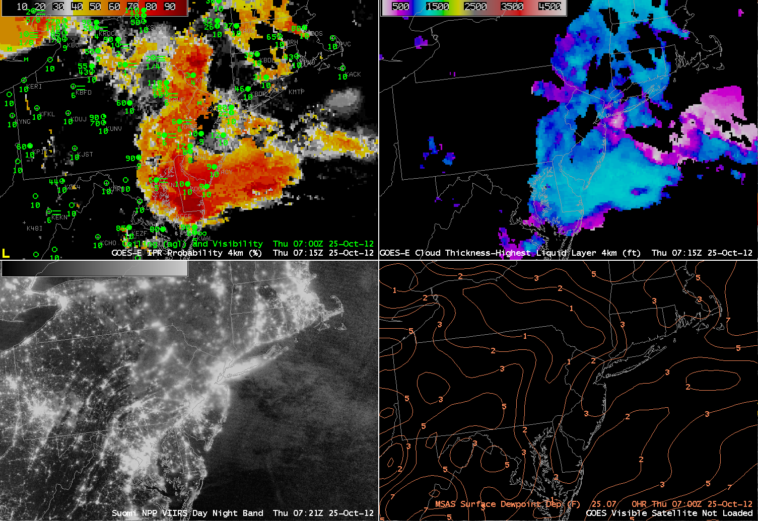
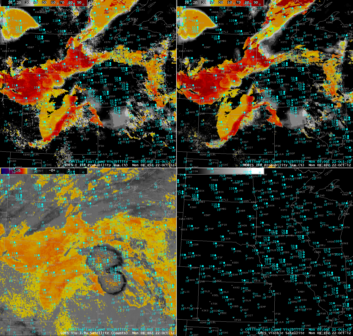
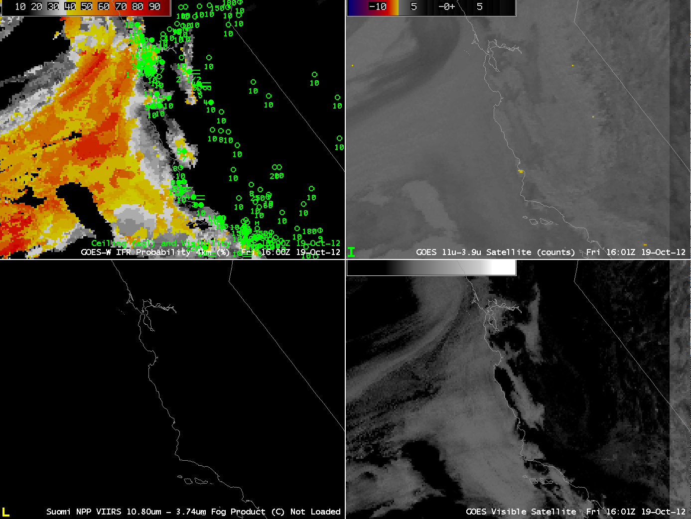
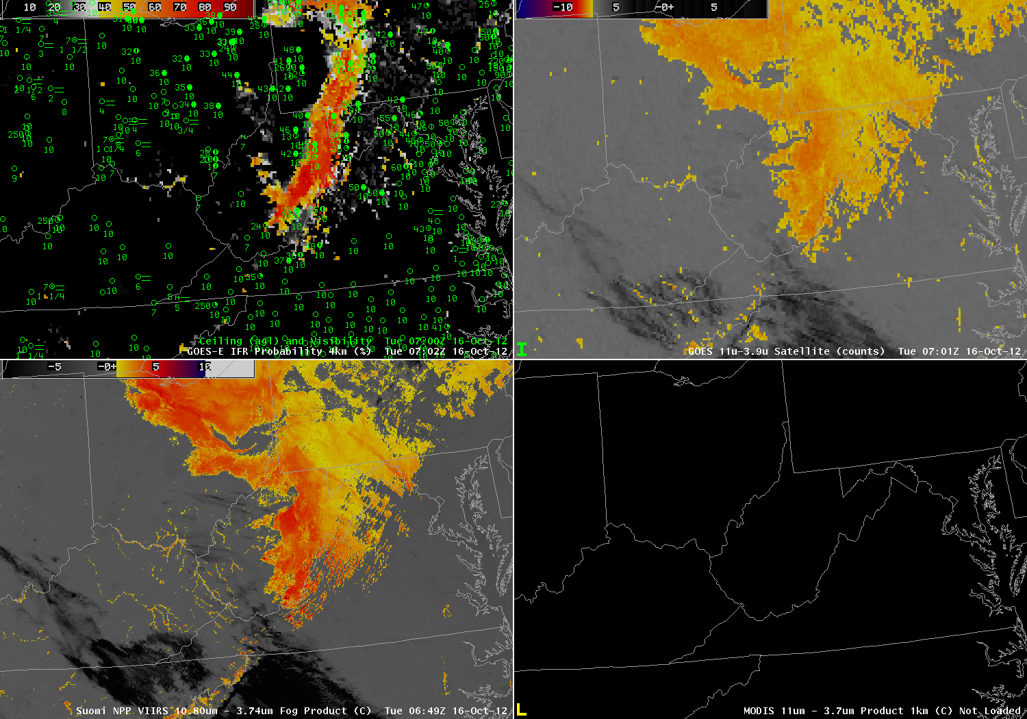
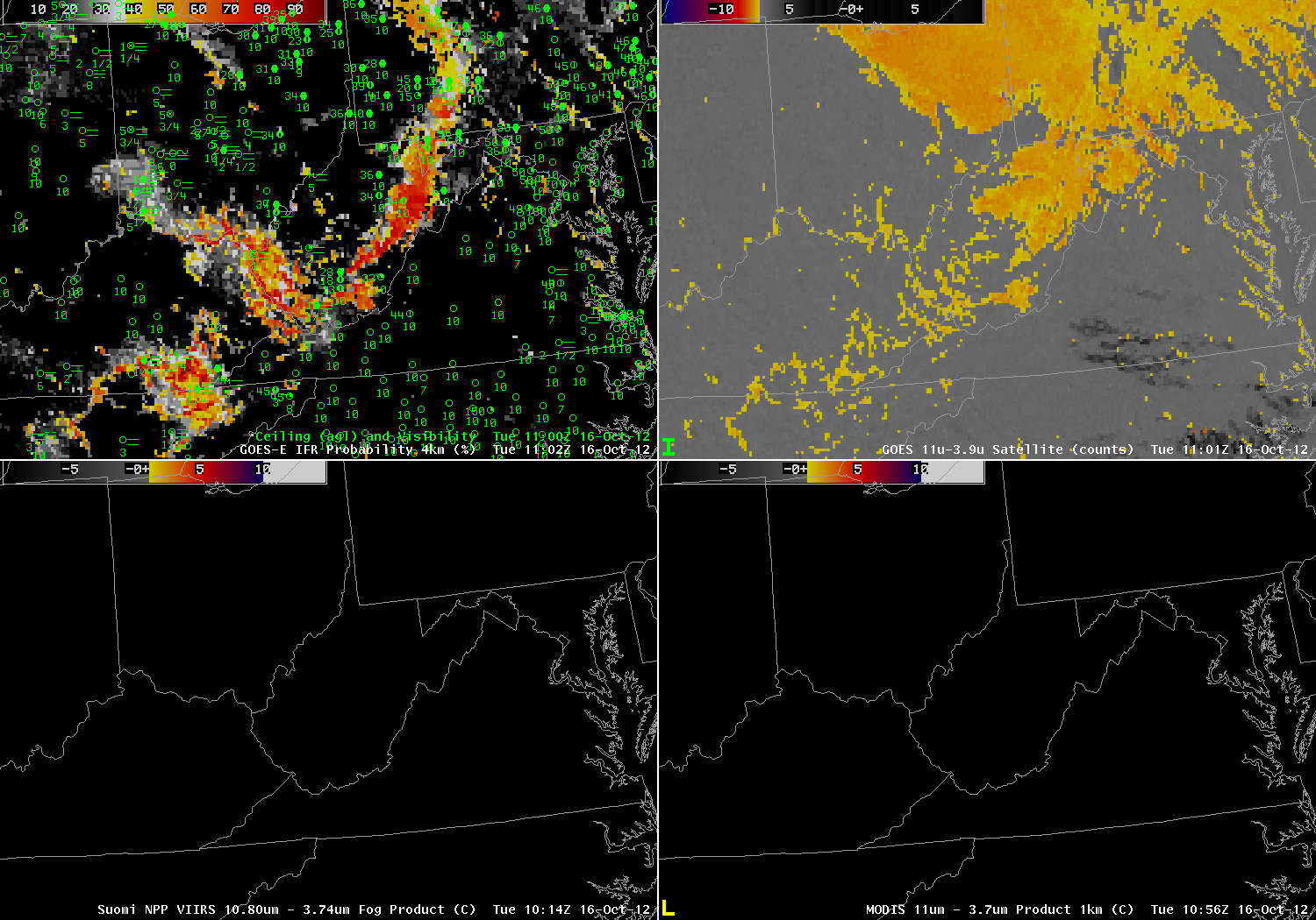
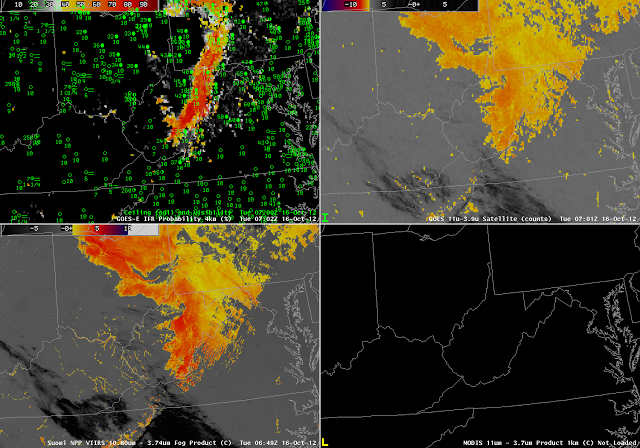
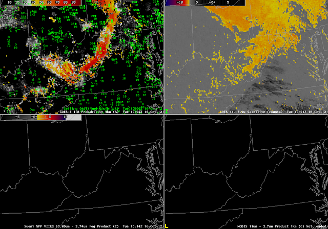
GOES-R IFR Probabilities computed from GOES-14 (upper left), GOES-14 heritage brightness temperature difference product (upper right), VIIRS heritage brightness temperature difference product (lower left), MODIS heritage brightness temperature difference product (lower right), all from near 0700 UTC.

MODIS and VIIRS yield satellite information that can be used to detect fog/low stratus at high spatial resolution.  In the exa,ple above, the VIIRS brightness temperature difference product highlights many river valleys as possibly cloud-filled over eastern Kentucky, southern Ohio and southwestern West Virginia.  The coarser resolution of the GOES satellite pixel precludes such fine-scale detection.  Note, however, that both satellite platforms detect the presence of stratiform water clouds over north-central Ohio where surface observations show only mid-level cloudiness.  IFR probabilities are confined to the spine of the Appalachians from the Laurel Mountains near Johnstown (PA) southward towards southern West Virginia.  How do things evolve with time?

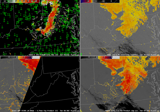
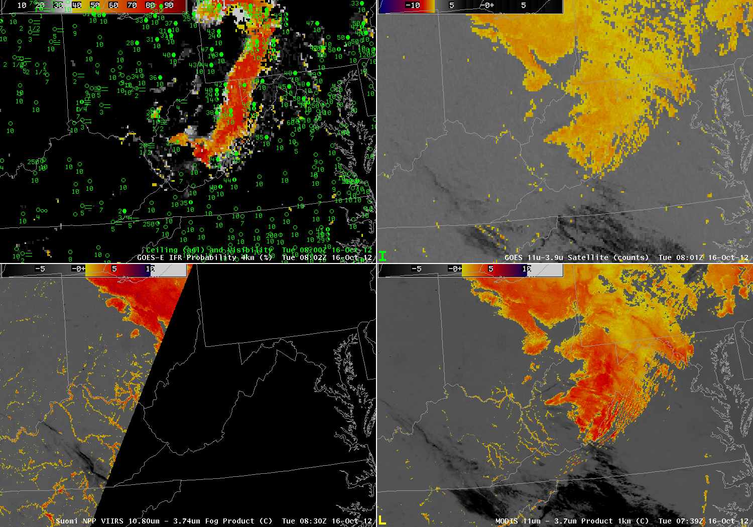
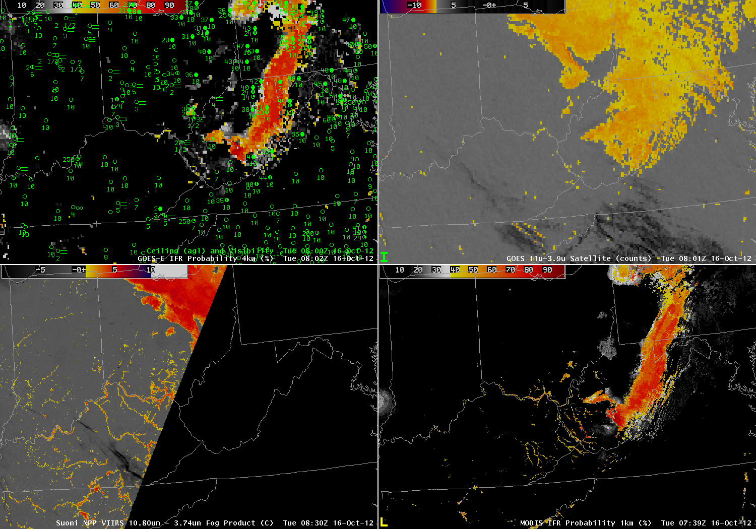
As above, but from near 0800 UTC

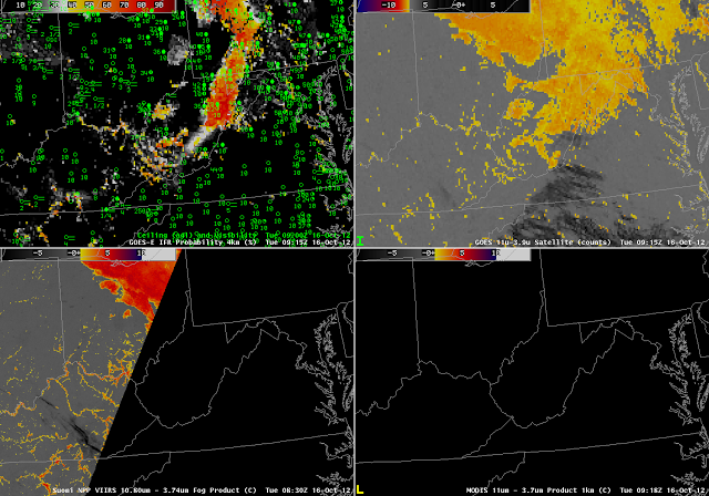
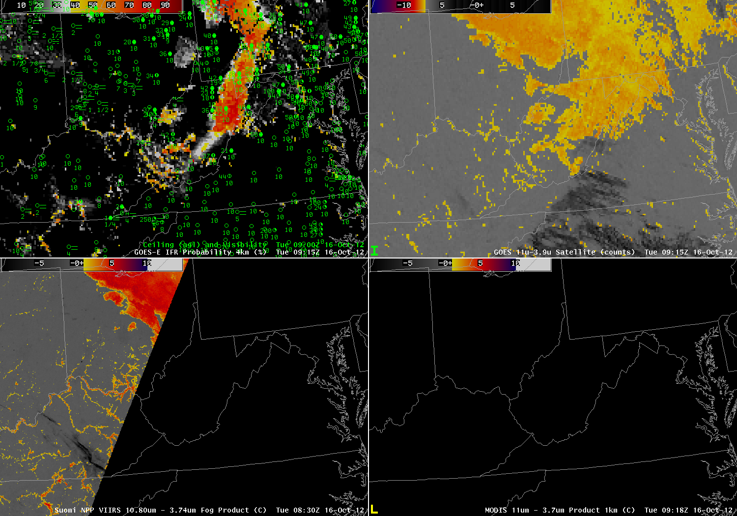
As above, but from near 0915 UTC

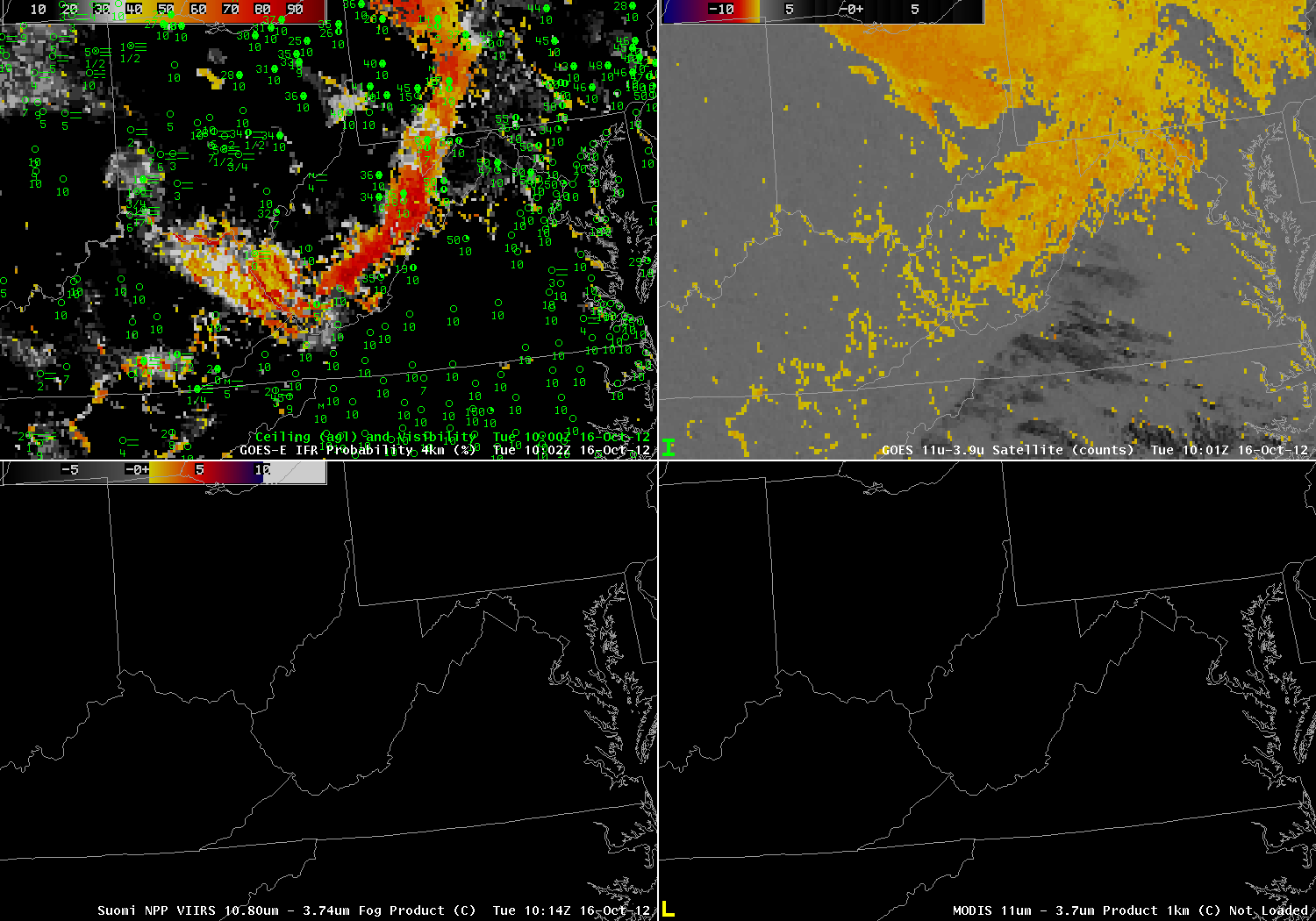
As above, but from near 1000 UTC

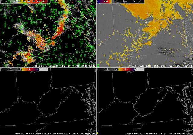
As above, but from near 1100 UTC

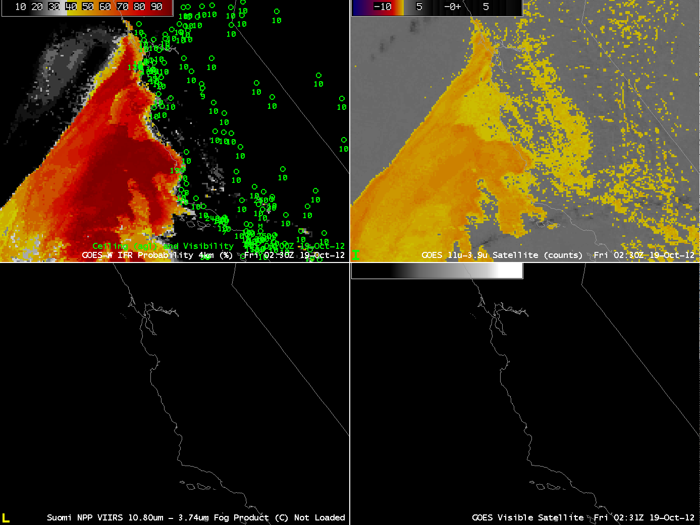
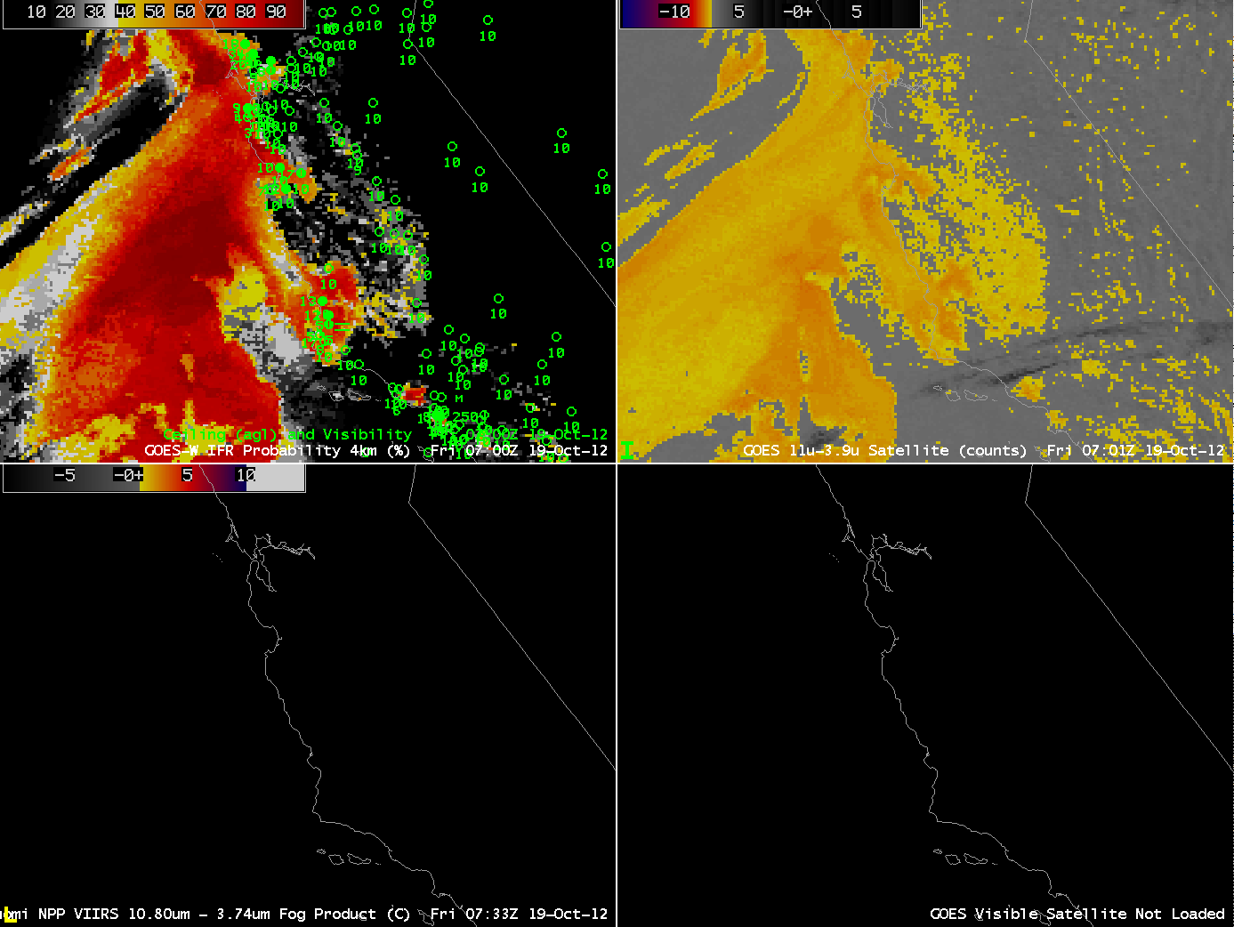
The power of GOES imagery in this case is to show the evolution of the fog/low stratus field.  Even at this only-hourly timestep, the development of regions of IFR conditions is evident, and those developing conditions occur in tandem with increasing probabilities in the GOES-R IFR Probability field.  Throughout the night, the GOES brightness temperature difference field flags the unimportant (from an aviation standpoint) stratus deck over northcentral Ohio, and the IFR probability field, which field also uses Rapid Refresh Model data, discounts the satellite signal.  By 1100 UTC, the river valley signal has strengthened enough in the GOES imagery to appear, and a corresponding increase in IFR probability occurs.

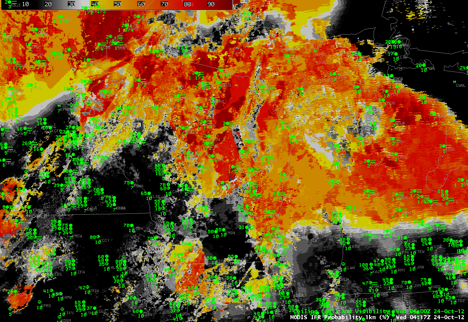
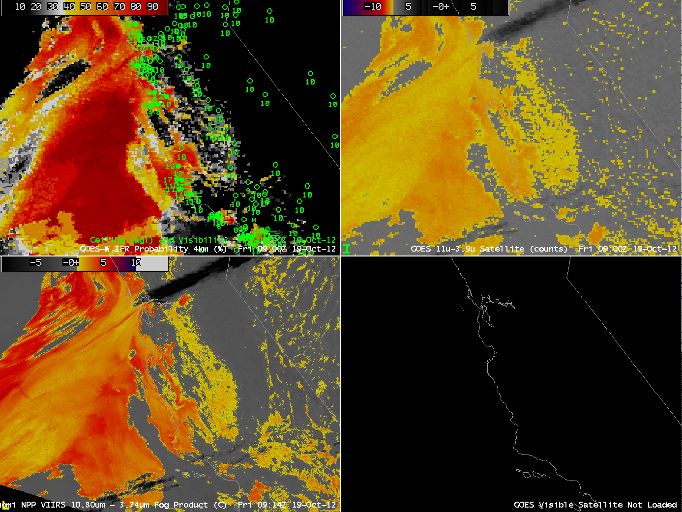
IFR Probability can also be computed using MODIS data (below). The 0739 UTC MODIS data, shown at the top of this blog post, highlights — as does GOES — the stratus deck over northern Ohio.  The MODIS-based IFR probabilities, however, do not highlight that cloud-deck, by design.  Note also that the higher-resolution MODIS imagery, because it detects river valley fogs at 0739 UTC, also has a strong IFR probability signal there.  Pixel resolution on GOES-R will be intermediate between MODIS and present GOES.

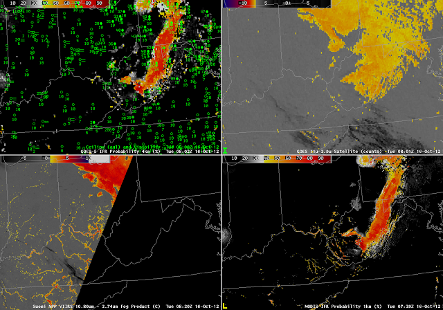
As at top, for near 0800 UTC, but with MODIS-based IFR probabilities in the lower right

Day/Night band and fog detection

Day/Night band from VIIRS on Suomi/NPP from 0714 UTC on 4 October 2012

The day/night band imagery, above, shows fog/low clouds in the Hill Country west of San Antonio and Austin in south-central Texas.  Additionally, there are low clouds over the Gulf of Mexico, with cloud street structures that suggest a south-southeasterly wind bringing moisture inland from the Gulf.  The 0855 UTC day/night band image over the same domain, below, shows an expansion of the fog/low cloud signal.

Day/Night band from VIIRS on Suomi/NPP from 0855 UTC on 4 October 2012
Day/Night band from Suomi/NPP with observations overlain.

Observations suggest that the northern edge of the cloud streets over the extreme western Gulf of Mexico is the edge of a moisture gradient, and that that gradient extends inland to where the fog and low stratus are occurring.  How did the GOES-R IFR Probability field perform on this day?  The 0702 UTC (below) and 0915 UTC IFR probability fields show an increas in the areal extent of higher probabilities over the course of the night, consistent with the overnight cooling and the continued feed of moisture from the Gulf.  By 0900 UTC, IFR observations are common in and near the region where IFR probabilities are high.  This is a good example of how the Day/Night band and IFR Probabilities can be used in concert to understand the evolution of the fog/low stratus field over south Texas.