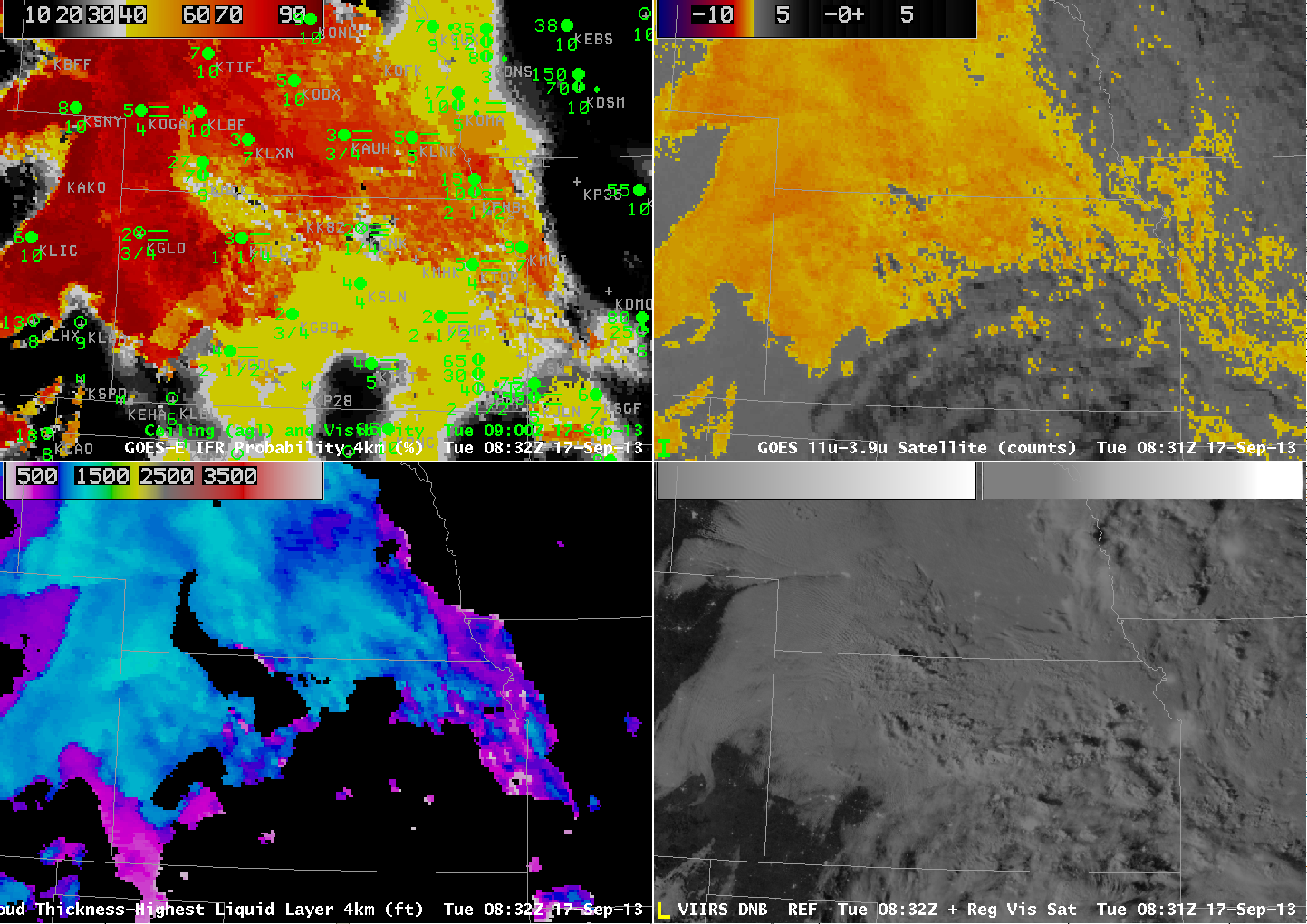
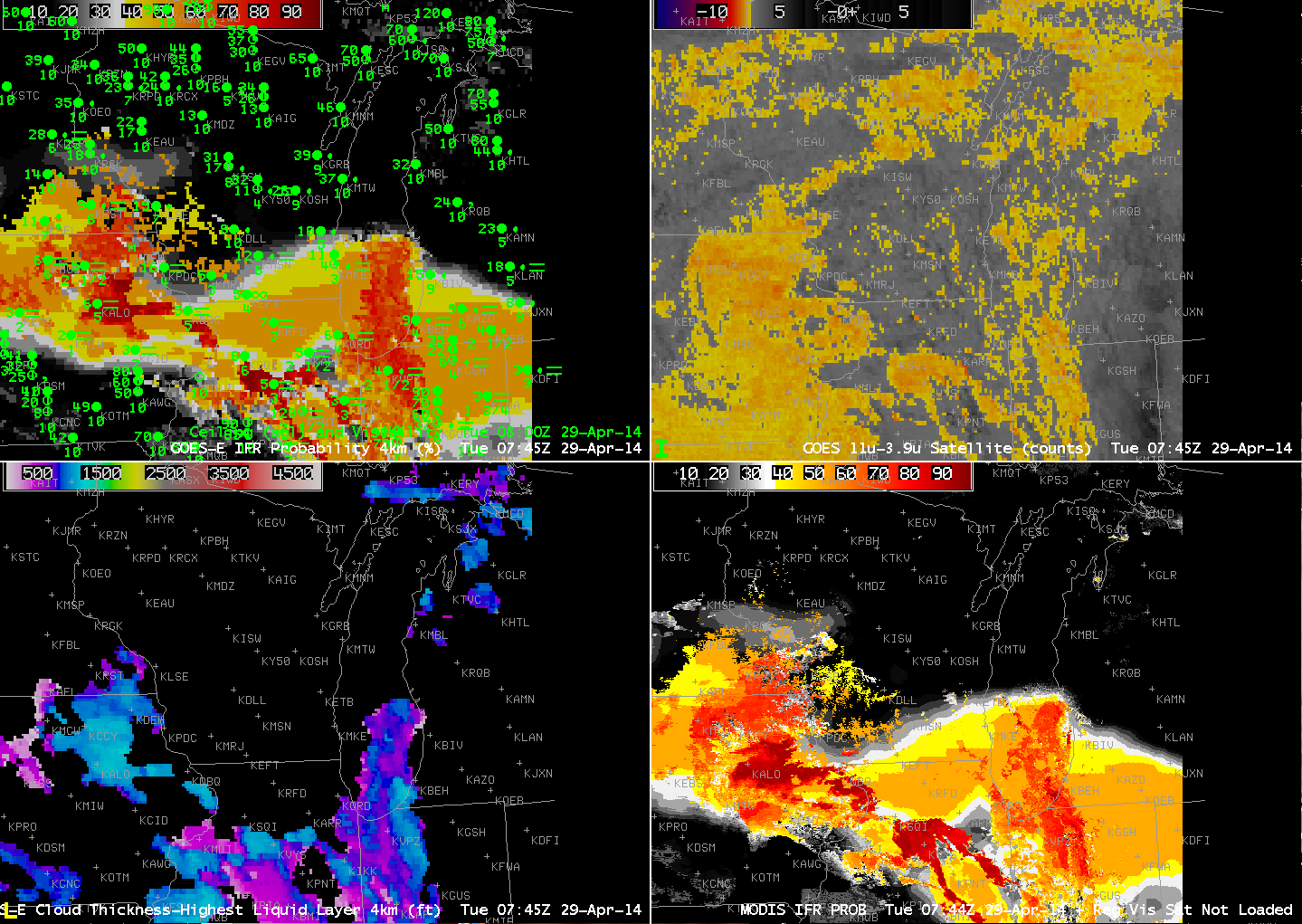
GOES-R IFR Probabilities from GOES-13 (Upper Left), GOES-13 Brightness Temperature Difference Product (10.7 µm – 3.9 µm) (Upper Right), GOES-R Cloud Thickness from GOES-13 (Lower Left), MODIS-based IFR Probabilities (Lower Right), Times as indicated (click image to enlarge)
Dense Fog developed over the southern Plains overnight, and the case demonstrates how the Fused data product is able to give a useful signal of IFR probabilities even in regions where high clouds preclude the detection of low clouds by satellite. The fog was widespread and dense enough to warrant Dense Fog Advisories from Tulsa, Norman and Topeka forecast offices. See below, for example.
000
FXUS64 KTSA 020953
AFDTSA
AREA FORECAST DISCUSSION
NATIONAL WEATHER SERVICE TULSA OK
353 AM CST MON DEC 2 2013
.DISCUSSION…
DENSE FOG CONTINUES THIS MORNING ACROSS MUCH OF THE CWA. GIVEN THE
TIME OF YEAR /LOW SUN ANGLE/ AND THE FACT THAT SOME HIGH CLOUDS ARE
STREAMING INTO THE AREA FROM THE NW /REDUCED INSOLATION AND
DELAYED MIXING/…THINK IT MAY TAKE A LITTLE LONGER THAN
PREVIOUSLY EXPECTED TO GET RID OF THE FOG. WE HAVE EXTENDED THE
DENSE FOG ADVISORY UNTIL 11 AM. ONCE THE FOG BURNS OFF…SHOULD
BE A PLEASANT DAY WITH UNSEASONABLY WARM TEMPS AND FAIRLY LIGHT
WIND. COULD BE SOME MORE FOG TUESDAY MORNING IN SOME PLACES BUT A
LITTLE MORE WIND MAY KEEP IT FROM GETTING AS DENSE AND AS
WIDESPREAD AS IT IS THIS MORNING. SLIGHTLY WARMER TEMPS IN STORE
TUESDAY WITH SOME PLACES LIKELY IN THE 70S. WARM AND WINDY
CONDITIONS WILL RESULT IN AN INCREASING FIRE WEATHER CONCERN.
Satellite detection of this fog event was constrained by the presence of two upper-level cloud decks. At the beginning of the animation, above, high clouds associated with the subtropical jet are over the southern quarter of the domain plotted. These high clouds quickly shift southward, and the region in the brightness temperature difference product that is consistent with detection of fog/low stratus (that is, low water-based clouds) expands to the south (surface observations suggest the low stratus clouds were present earlier, but masked by the higher clouds). Later in the animation, high clouds sag southward into the northern part of the domain. When this happens, low stratus/fog (indicated in observations by IFR conditions) are not detected by GOES because the higher ice clouds block the view of the scene. However, the IFR Probability fields that use both satellite data and output from the Rapid Refresh Model continue to depict a likely region (confirmed by the observations) of reduced visibilities. IFR Probabilities do drop, of course, as satellite data cannot be used to confirm the presence of low clouds. Knowledge of why the probabilities drop is vital to the interpretation of the field: You have to know that the high clouds are present, either by looking at the satellite data, or by understanding that the character of the IFR Probability field changes to one that is less pixelated when satellite data cannot be included because of ice clouds above the low stratus deck.

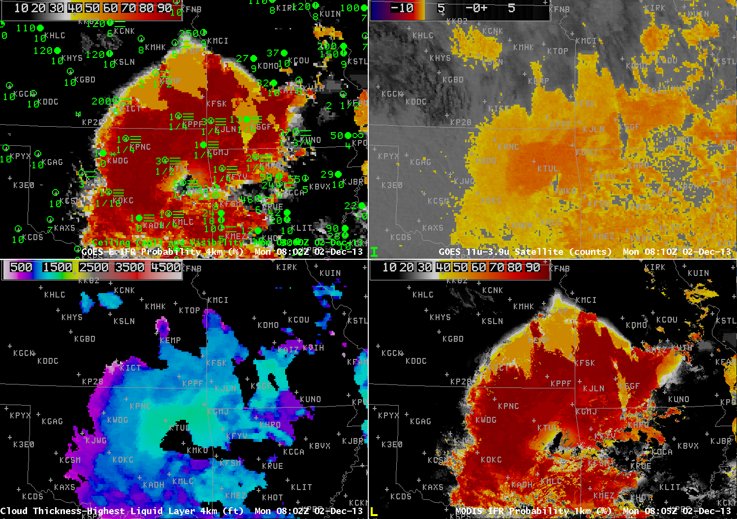
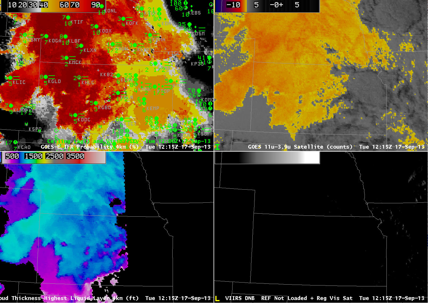
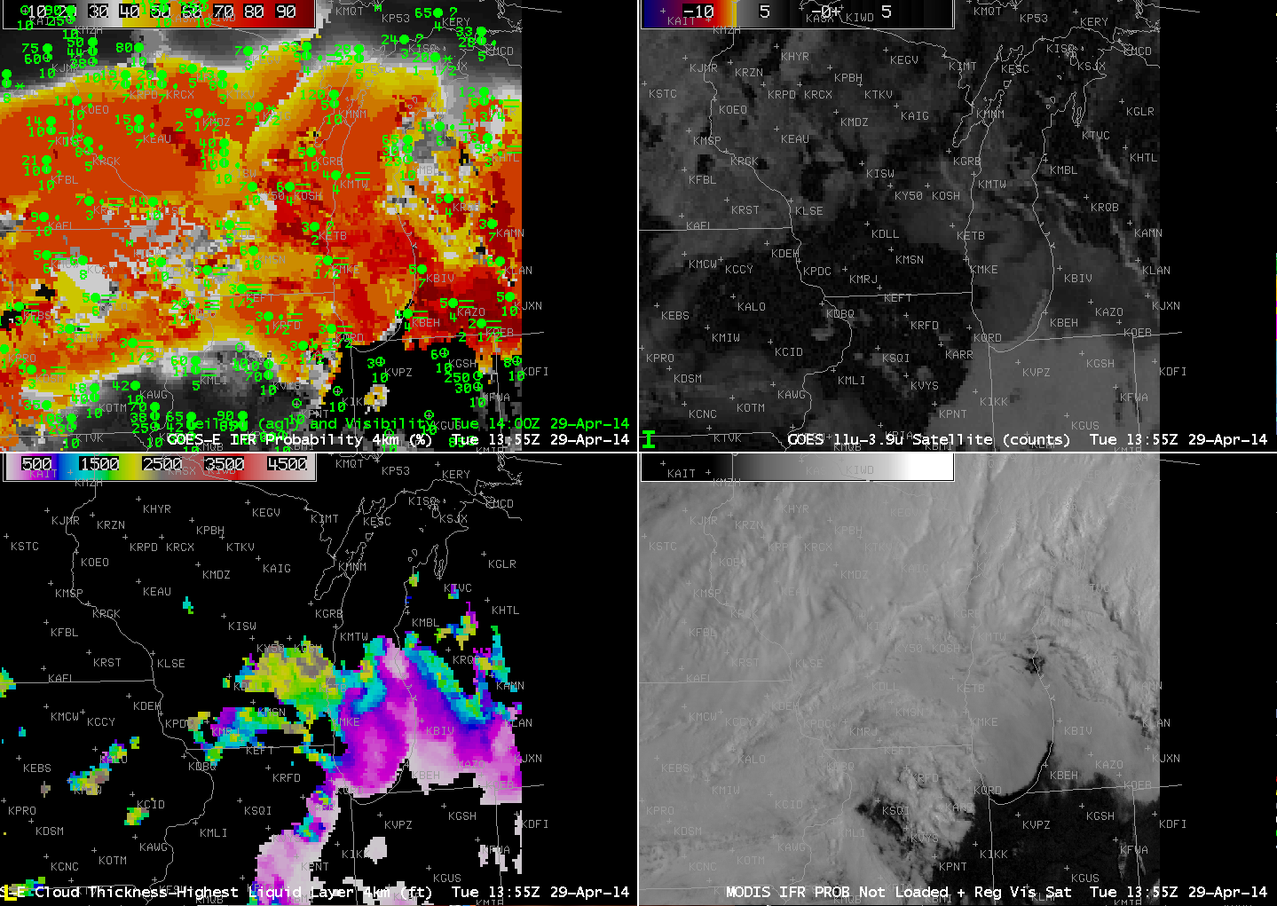
GOES-R IFR Probabilities from GOES-13 (Upper Left), GOES-13 Brightness Temperature Difference Product (10.7 µm – 3.9 µm) (Upper Right), GOES-R Cloud Thickness from GOES-13 (Lower Left), MODIS-based IFR Probabilities (Lower Right), Times near 0802 UTC as indicated (click image to enlarge)
For a large-scale event like this, MODIS-based IFR Probabilities overlap well with GOES-Based IFR Probabilities, as shown in the image above. In cases like this sometimes individual river valleys will show up with slightly elevated IFR Probabilities (or cloud thicknesses).
The GOES-R Cloud Thickness field is computed for the highest water-based cloud detected (during non-twilight conditions — that is, not during the hour or so surrounding sunrise and sunset). Note how well the thickest clouds — over northeast OK, surrounding Tulsa — correlate with the strongest Brightness Temperature Difference, both in GOES and in Suomi/NPP data (below). Note also how the Cloud Thickness field is not computed in regions where higher ice-based clouds are present.
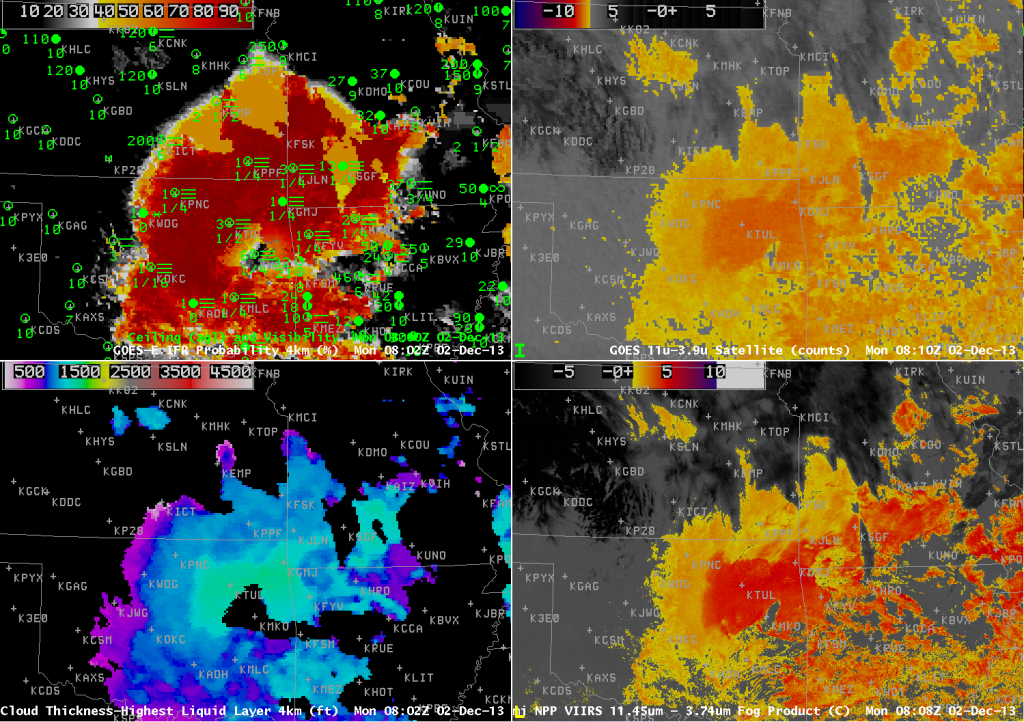
GOES-R IFR Probabilities from GOES-13 (Upper Left), GOES-13 Brightness Temperature Difference Product (10.7 µm – 3.9 µm) (Upper Right), GOES-R Cloud Thickness from GOES-13 (Lower Left), Suomi/NPP Brightness Temperature Difference from VIIRS (10.35 µm – 3.74 µm) (Lower Right), Times near 0802 UTC as indicated (click image to enlarge)
Cloud Thickness can be used to predict the time of fog dissipation, using this scatterplot/relationship. If sun angle is limited by the season, or if solar insolation is limited by higher clouds, you might adjust the first guess for dissipation to a later time.


