Author Archives: Scott Lindstrom

Interpreting IFR Probability Fields

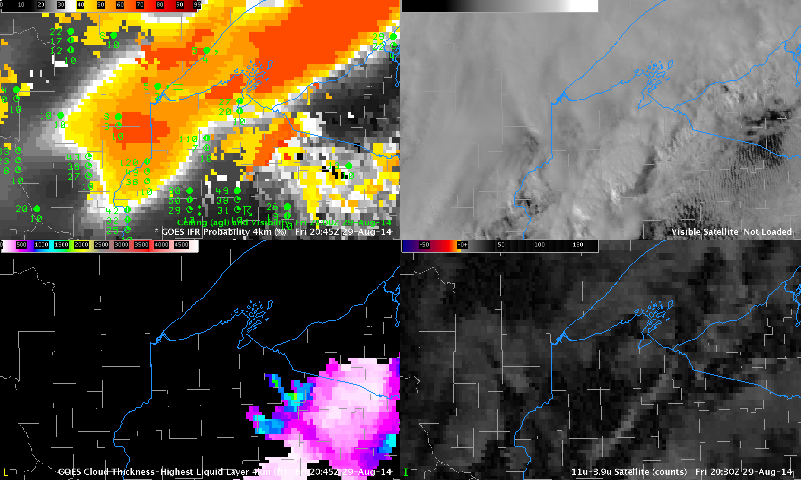
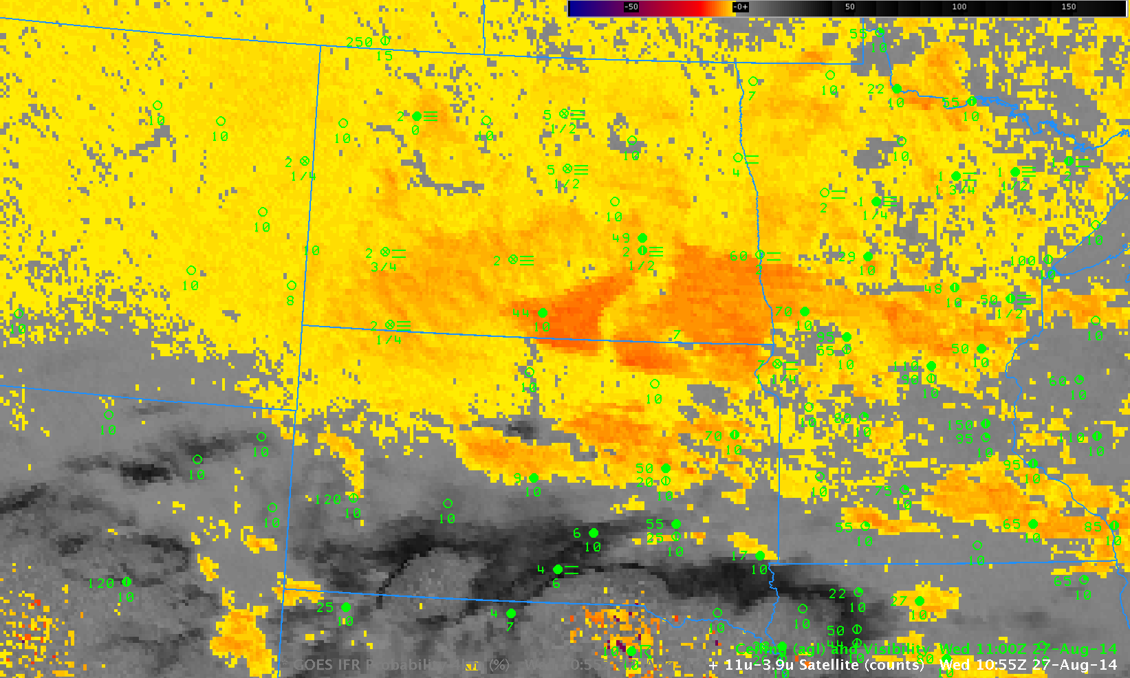
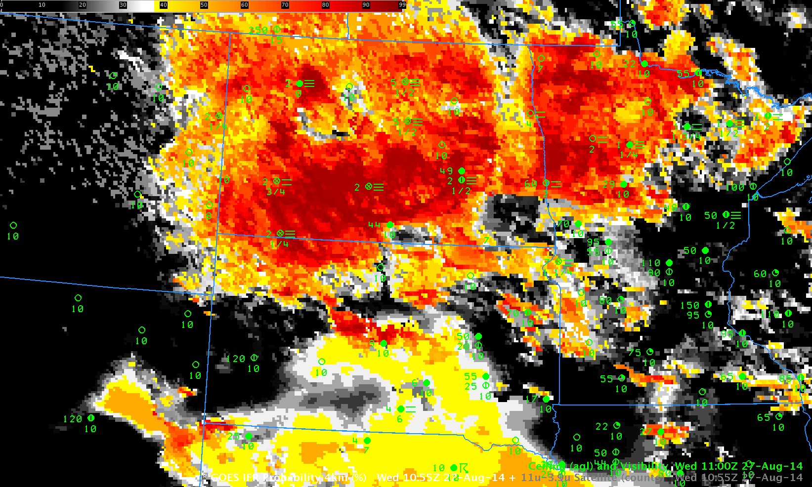
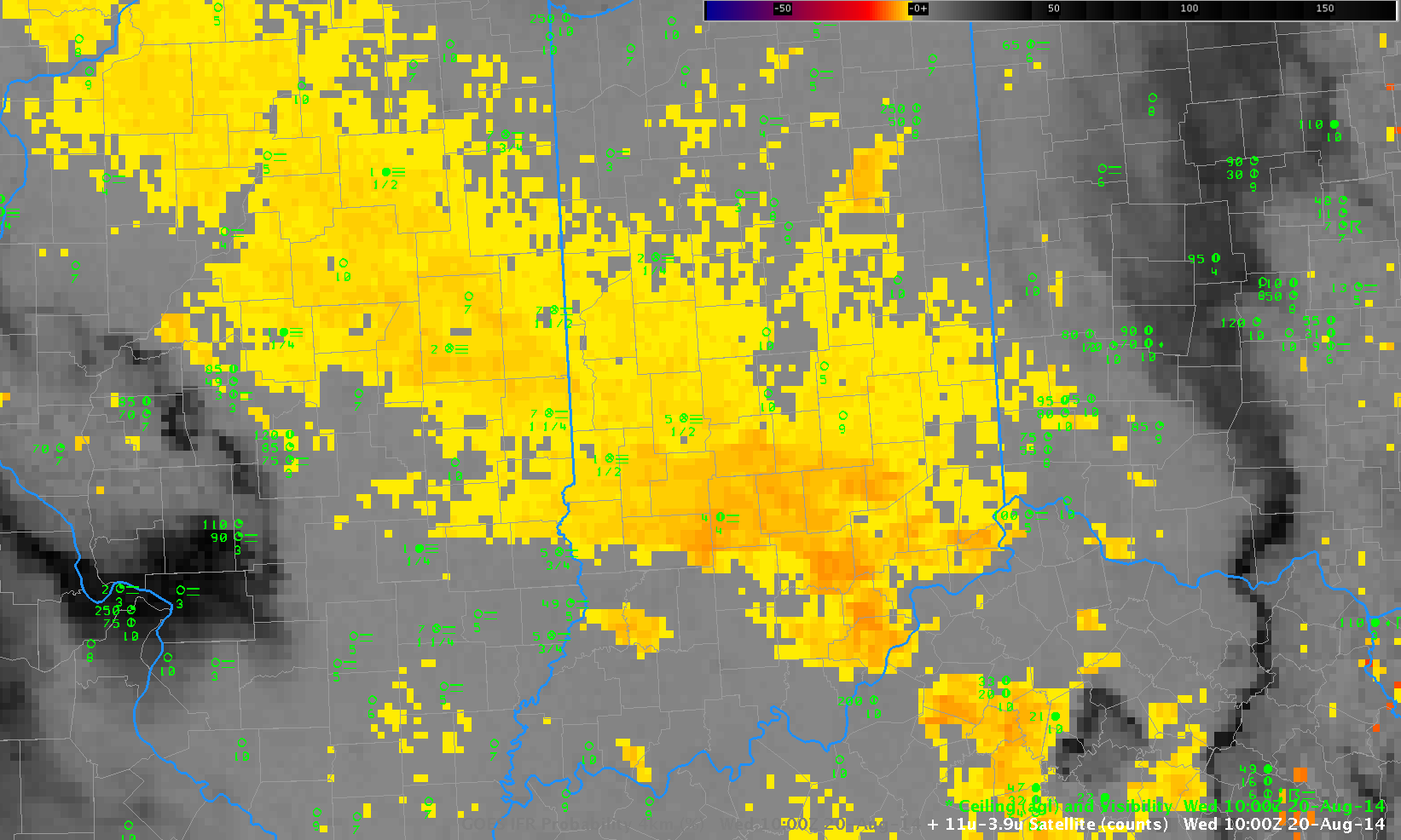
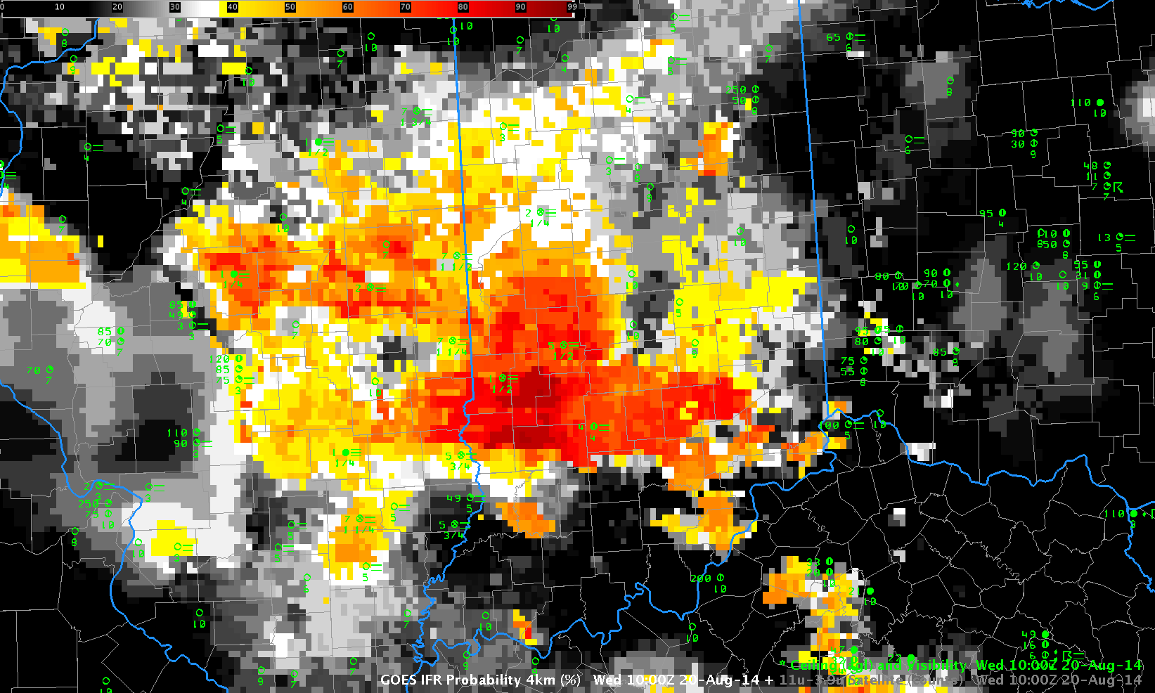
Toggle between GOES-R IFR Probabilities and GOES-East Brightness Temperature Differences (10.7 µm – 3.9 µm) over the southeast US, 0700 UTC 8 September 2014 (Click to enlarge)

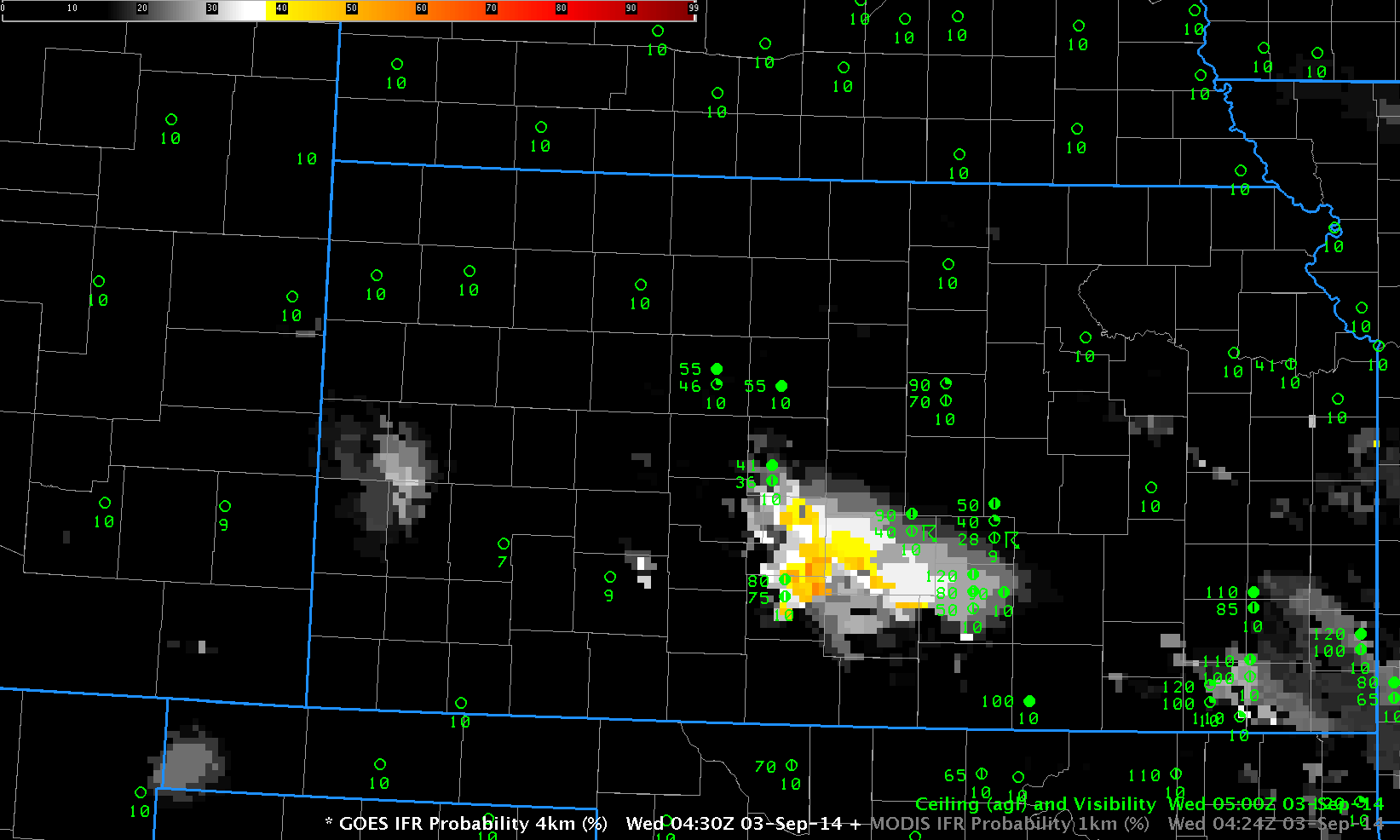
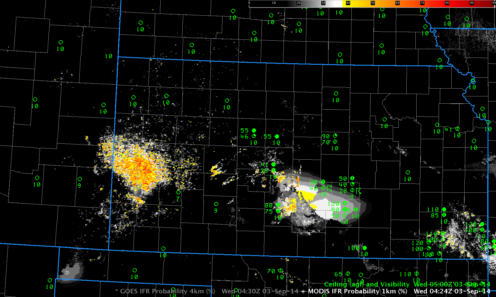
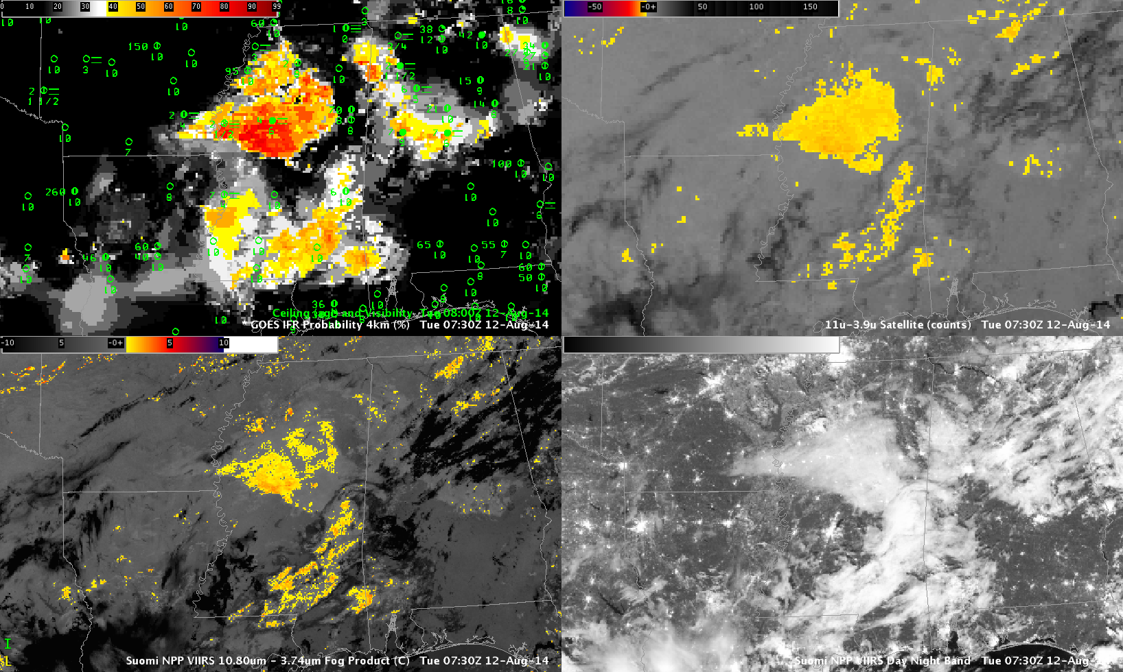
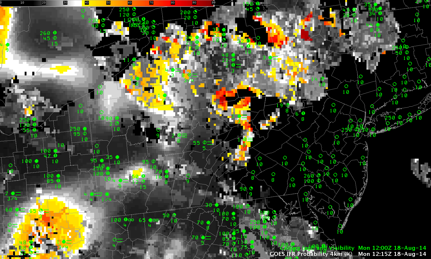
When multiple cloud layers are present, such as when a cirrus shield overlays a region, the traditional method of detecting fog/low stratus, the brightness temperature difference product, struggles to identify regions of low clouds because the satellite sees only the signature of the high clouds. Low clouds are hidden from view. In such cases, it is vital to incorporate low-level information to identify regions where fog/low stratus might be present. The required low-level information can come from the model fields of the Rapid Refresh Model. The model predictors can be used to generate IFR Probabilities in regions where satellite predictors are unavailable because of the presence of high clouds.

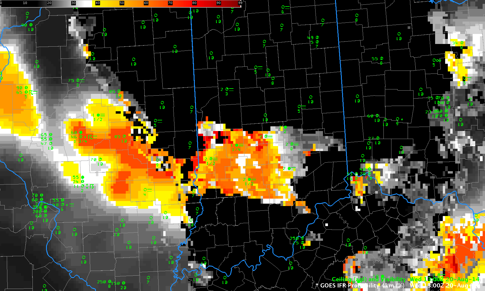
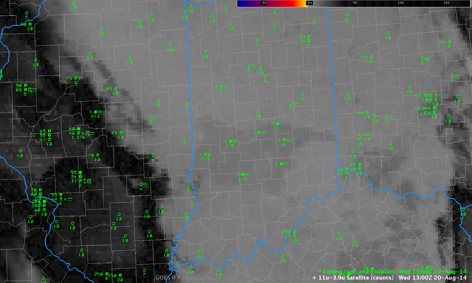
In the toggle above, the Brightness Temperature Difference field shows high clouds over Georgia and the Carolinas. IFR Probabilities in this region are around 50% — relatively low because Cloud Predictors cannot be used in the algorithm. But IFR Conditions are present over North and South Carolina. Tailor your interpretation of the IFR Probability values to account for which predictors are used.

Over Tennessee, IFR Probabilities are much higher. In this region, satellite predictors can be used, and a strong satellite signal is present. IFR Conditions are not widespread, however. Use the IFR Probability field as one tool (but not the only tool) when making nowcasts about the possibilities of fog/low stratus.

MODIS-based and GOES-based IFR Probabilities over the High Plains

GOES-based GOES-R IFR Probabilities over Kansas and surrounding states, 0430 UTC 3 September 2014 (Click to enlarge)

GOES-based IFR Probabilities over Kansas before midnight on 2 September highlight two regions where IFR Conditions might be developing: over western Kansas, near the Colorado border, and over south-central Kansas. These would be two places to monitor most closely over the coming hours. The MODIS-based IFR Probabilities for the same time, below, can be used to refine the interpretation of the GOES fields. IFR probabilities over western Kansas are higher with the MODIS data. IFR Probabilities from MODIS better capture the difference in the field over south-central Kansas as well: there is a more obvious distinction between IFR Probabilities influenced solely by model output (because of the multiple cloud layers associated with the thunderstorm at Hutchinson and Newton) and those controlled by both model and satellite predictors. The strength of GOES-based IFR Probabilities is temporal continuity. How do the fields evolve with time?

MODIS-based GOES-R IFR Probabilities over Kansas and surrounding states, 0424 UTC 3 September 2014 (Click to enlarge)

The animation below of GOES-based IFR Probabilities shows increasing values over western Kansas (the region drifts northward, as well); by 1045 UTC, at the end of the animation, IFR Probabilities are very high over western and northwestern Kansas, and IFR conditions are observed in the form of both low ceilings and reduced visibilities. This was a case where MODIS data gave an early alert to where GOES-based IFR probabilities might later become high. Fog can start at small scales and then grow in size and MODIS data offers an advantage of higher spatial resolution. A toggle between the MODIS and GOES-based IFR Probabilities at 0836 UTC is at bottom.

GOES-based GOES-R IFR Probabilities over Kansas and surrounding states, times as indicated on 3 September 2014 (Click to enlarge)

MODIS- and GOES-based GOES-R IFR Probabilities over Kansas and surrounding states, 0836 UTC on 3 September 2014 (Click to enlarge)

IFR Probabilities over the Texas Panhandle

GOES_MODIS_IFR_SNPP_BTD-DNB_0930UTC_02Sep2014

GOES-R IFR Probabilities (Upper Right), GOES-13 Brightness Temperature Difference (10.7 µm – 3.9 µm) (Upper Left), MODIS IFR Probabilities (Lower Left), Suomi NPP Brightness Temperature Difference (11.35 µm – 3.74 µm) and Day Night Band (Lower Right), all near 0930 UTC 2 September 2014 (Click to enlarge)

GOES-R IFR Probabilities (from GOES and from MODIS) over the Great Plains and southern Rockies indicated one region where IFR conditions were most likely: over the Texas panhandle, where IFR conditions were reported. There is a strong signal in the GOES-based Brightness Temperature Difference field there (and in the Suomi NPP Brightness Temperature Difference field) as well. There is also a Brightness Temperature difference signal in regions where IFR conditions are not occurring; in those locations, stratus is present, or (over the Rockies) emissivity differences in the dry soil are present, both of which conditions will lead to a signal in the brightness temperature difference that is unrelated to surface visibility and ceilings. This is therefore another example showing how incorporation of model data that accurately describes saturation (or near-saturation) in the lowest model layers can help the GOES-R IFR Probability more accurately depict where IFR conditions are present.

IFR Conditions under multiple cloud layers

GOES-R IFR Probabilities with surface observations of ceilings and visibilities (Upper Left), GOES-East Visible Image (Upper Right), GOES-East Brightness Temperature Difference (10.7 µm – 3.9 µm) (Lower Right), GOES-R Cloud Thickness (Lower Left), all near 2100 UTC (Click to enlarge)

IFR and near-IFR conditions existed near Duluth Minnesota during the day on 29 August 2014; How does information from the satellite help to diagnose the IFR conditions? Both the visible and brightness temperature difference fields, above, show widespread cloudiness, with convective features over Wisconsin and multiple cloud decks over Wisconsin and Minnesota. These multiple cloud decks show no apparent relationship the observed IFR or near-IFR conditions. In cases such as these, the low-level information available through the Rapid Refresh Model is key to providing information defining exactly where the lowest ceilings and visibilities exist. In the case above, that region is centered near Duluth, extending to the southwest. IFR Probabilities are elevated in regions where visibilities and ceilings are low, and they increase as the cloud ceiling increases. The image below shows Duluth Harbor at about 2140 UTC; the low ceiling is apparent (Source).

Fog and Stratus over the Dakotas

GOES Brightness Temperature Difference (10.7 µm – 3.9 µm) and surface observations of ceilings and visibilities, 1100 UTC, 27 August 2014

GOES data indicated widespread stratus over North Dakota and adjacent states early in the morning on 27 August. The image above demonstrates several difficulties that come with using the brightness temperature difference field to identify regions of reduced ceilings and visibilities. A stratus deck (over eastern Montana) and a fog bank (over central North Dakota) can have a very similar signal in the brightness temperature difference field. Furthermore, regions where ice crystals comprise the clouds (southern South Dakota) show a different signal. Low-level stratus will be invisible to the satellite at night if it is beneath a higher-level cirrus shield.

IFR Probabilities for the same time, below, more accurately define where the lowest visibilities and ceilings occur because Rapid Refresh Model data are used to identify regions where part of the lowest layers of the model atmosphere is saturated. If there is saturation below higher clouds (southern South Dakota), then IFR Probabilities are increased. If there is not low-level saturation in the model in regions where low stratus/fog is present, then IFR Probabilities are reduced (eastern Montana).

Note also how the character of the fields changes if satellite data are not used as an IFR Probability predictor. IFR Probabilities in southern South Dakota (where multiple cloud layers are present associated with a convective feature) have a uniform look to them, as they are derived solely from model-based fields. Over North Dakota and Montana, satellite data can be used as a predictor; the individual satellite pixels are obvious. When only model data are used as predictors, the probability is reduced. Thus, the color yellow in a region of model-only prediction (southern South Dakota) should be interpreted differently than the color yellow in a region that uses both model and satellite predictors (North Dakota and Montana).

GOES-R IFR Probabilities and observations of ceilings and visibilities, 1100 UTC, 27 August 2014

Fog over Indiana

GOES-R IFR Probabilities computed from GOES-13 data, 1300 UTC 20 August 2014

A small area of IFR conditions developed over southern Indiana during the overnight/early morning hours of 20 August, and the imagery in this post serves as a good tutorial for how to interpret GOES-R IFR Probabilities. The 1300 UTC imagery, above, is from after sunrise; therefore, the cloud-clearing algorithm (that includes visible imagery) will do a good job of screening out regions where widespread fog is not present (Compare this image to the 1000 UTC image that cannot use visible imagery below). The highest IFR Probabilities are confined to the region over southern Indiana where ceilings and visibilities are near or below IFR conditions. The effect of a large convective complex with multiple cloud layers on the IFR probabilities is apparent over Illinois. There, IFR Probabilities have a very smooth appearance because satellite predicitors (which predictors can be pixelated in appearance) are not used: only model data are driving the IFR Probability over most of Illinois. The Brightness Temperature Difference field, below, (10.7 µm – 3.9 µm), the heritage method of identifying regions of low clouds, displays the difficulty inherent in the field after sunrise: solar radiation with a wavelength of 3.9 µm changes the character of the difference field, making interpretation difficult.

GOES-13 Brightness Temperature Difference Field (10.7 µm – 3.9 µm) 1300 UTC 20 August 2014

The GOES-13 Brightness Temperature Difference field at 1000 UTC, below, has a more characteristic look for a scene with fog and low stratus present. However, the signal overpredicts where reduced ceilings/visibilities are actually occurring. Mid-level stratus and fog can look very similar when viewed from a satellite. The IFR Probability field at the same time (1000 UTC), at bottom, has highest probabilities over the region of IFR conditions — over southern Indiana. Some regions with a strong Brightness Temperature Difference signal — for example, in western Illinois near Moline/Davenport — have a comparatively weak IFR Probability signal. In those regions, the Rapid Refresh model is correctly suggesting that low-level saturation is unlikely.

GOES-13 Brightness Temperature Difference Field (10.7 µm – 3.9 µm) 1000 UTC 20 August 2014

GOES-R IFR Probabilities computed from GOES-13 data, 1000 UTC 20 August 2014

Fog over Pennsylvania

GOES-R IFR Probabilities computed from GOES-13 data, hourly from 0500 through 1300 UTC 18 August 2014

River valley fog developed over Pennsylvania during the early morning hours of 18 August 2014, and the case is a good test of the GOES-R IFR Probability fields. IFR Probabilities are low at 0500 UTC (1 AM local time) and subsequently increase rapidly. In this case, the fields may be overpredicting where fog is present, as visible imagery just after sunrise suggest it was confined mostly to river valleys. In the animation above, the areal extent of the IFR Probabilities drops between 1100 UTC and 1215 UTC as the sun rises (the terminator is apparent in the 1100 UTC image, running from western Maryland north-northwestward to extreme western New York) and visible imagery can be used to more effectively cloud-clear the fields. A toggle between these two times is below. In this case, it is important to understand the geography underneath the IFR Probability field to hone the forecast.

GOES-R IFR Probabilities computed from GOES-13 data, at 1100 and 1215 UTC 18 August 2014

GOES-East Brightness Temperature Difference Fields (10.7µm – 3.9µm), hourly, from 0500-1100 UTC 18 August 2014

The Brightness Temperature Difference field, above, is the heritage method of detecting low stratus and inferring the presence of fog. Interpretation is complicated because high clouds (initially present over the southwestern portion of the scene, and moving eastward) prevent the satellite from viewing low clouds. In addition, as the sun rises (at the end of the animation, at 1100 UTC), solar radiation changes the character of the the brightness temperature difference field.

Data from the MODIS on board both Terra and Aqua can also be used to create both brightness temperature difference fields and IFR Probability fields. The toggle below, using ~0700 UTC data from GOES and from MODIS, shows the distinct advantage present in the MODIS field’s superior spatial resolution (1-km at sub-satellite point vs. 4-km at the sub-satellite point for GOES). River valleys are more evident in the MODIS data, by far, than in the GOES data.

GOES-R IFR Probabilities computed from GOES-13 data and from MODIS data, at 0700 UTC 18 August 2014

The Day-Night band on Suomi NPP at 0718 UTC showed that the densest fog was largely confined to river valleys.

Suomi NPP Day/Night Band, 0718 UTC on 18 August 2014

An animation of the fog burning off from GOES-14 (in special 1-minute SRSO-R scanning operations) is available here. It’s also on YouTube.

Fog over Mississippi

GOES-R IFR Probabilities computed from GOES-13 at 0730 UTC (Upper Left), GOES-13 Brightness Temperature DIfference (10.7 µm – 3.9 µm) (Upper Right), Suomi NPP VIIRS Brightness Temperature Difference (11.35 µm – 3.74 µm) (Lower Left), Suomi NPP VIIRS Day Night Band (Lower Right), all at 0730 UTC on 12 August 2014

Fog developed overnight in central Mississippi, and the imagery above, at 0730 UTC, is a snapshot during the development. The just-past-full moon provided plenty of illumination, so the stratus and cirrus clouds over the south are distinct. It can be difficult, however, using only the Day Night Band to distinguish between low stratus (north-central Mississippi), mid-level stratus (eastern Mississippi), and high, thick cirrus (Alabama). In addition, the Day Night Band and the brightness temperature difference fields give information at the top of the cloud only. Information about the bottom of the cloud — whether the stratus deck extends to the surface as fog, for example, is difficult to glean from cloud-top properties. This is where the IFR Probability field that incorporates both cloud-top features derived from the brightness temperature difference field and lower-tropospheric information extracted from the Rapid Refresh Model can improve the detection of reduced ceilings and visibilities. Suomi NPP and other polar orbiters can give high spatial resolution imagery. GOES data has excellent temporal resolution to monitor how things evolve with time. The animation below shows how the fog/low stratus developed over the course of the day.

GOES-R IFR Probabilities and Surface observations of visibility/ceilings, hourly 0200-1100 UTC 12 August 2014

The fields in the animation above change character over the course of the night. Initially, the fields over southwestern Mississippi are very smooth; in this region, multiple cloud layers (a thunderstorm complex was dissipating) prevent any satellite signal from being used as a predictor for IFR Probabilities; only model data are being used. As the night progresses and the mid-level and upper-level clouds dissipate, the character of the field takes on a more pixelated appearance that means satellite data are being used as a predictor. The addition of satellite data to the suite of predictors also means that the probability value increases. By the end of the night, high probabilities have overspread much of central Mississippi, and low ceilings and reduced visibilities are widespread.

GOES-R Cloud Thickness can be used to estimate times of fog dissipation, using the relationship in this scatterplot and the Cloud Thickness in the last pre-sunrise scene, shown below for 12 August 2014. The thickest values are near Vicksburg, MS, where GOES-R Cloud Thickness approaches 1000 feet. That suggests a clearing time around 1400 UTC, ~3 hours after the valid time of the image below. The visible animation of the low clouds clearing is below.

GOES-R Cloud Thickness, 1100 UTC 12 August 2014

Fog in the Ohio Valley

GOES_OBS_BTD_SNPPBTD_MODISIFR_04August2014_0815

GOES-R IFR Probabilities and Surface observations of Ceiling and Visibility (Upper Left), GOES-East Brightness Temperature Difference (10.7 µm – 3.9 µm) (Upper Right), Suomi-NPP Brightness Temperature Difference (11.35 µm – 3.74 µm) (Lower Left), MODIS-based IFR Probabilities and Brightness Temperature Difference (11.0 µm – 3.9 µm) (Lower Right), all times as indicated

There are different ways to alert a forecaster to the presence of a transporation hazard like low ceilings and reduced visibilities. The imagery above shows GOES-based (nominal 4-km resolution at nadir) products (top) and Suomi/NPP and MODIS-based products (nominal 1-km resolution — or better — at nadir). The Brightness Temperature Difference from GOES (upper right) overestimates the region with lowered ceilings; in contrast, the IFR Probability field (upper Left) is able to distinguish between elevated stratus and low stratus because it includes information from the Rapid Refresh model to identify regions with saturation in the lowest levels of the atmosphere. This allows the IFR Probability to screen out regions of mid-level stratus.

The Suomi NPP and MODIS Brightness Temperature Difference fields do not suggest widespread stratus as does the GOES-based Brightness Temperature Difference field. Rather, the data from the polar orbiters suggest regions of stratus or fog in river valleys over Kentucky, Indiana and Illinois. MODIS-based IFR Probability (Lower Right) agrees with the GOES-based IFR Probability field: a region of fog/low stratus is developing over southwestern Indiana and southeastern Illinois, near the Wabash River. In this case, the model data is helping to strengthen a weak signal in a region where fog is present. Model data is a key strength in the IFR Probability field.

Polar orbiters give excellent horizontal resolution, but only GOES provides the high temporal resolution necessary to monitor the development of fog/low stratus. The toggle between 0800 and 1100 UTC, below, for example, depicts an increase in fog. A single GOES satellite can (and does) monitor that increase. A suite of polar orbiters would be required to give similar temporal coverage in middle latitudes.

As above, times as indicated

Fog and low stratus over the North Carolina piedmont

Hourly imagery of GOES-R IFR Probabilities over North Carolina, 0500-1400 UTC 23 July 2014, including surface observations of ceilings and visibilities

Low ceilings and reduced visibilities developed along the North Carolina piedmont during the morning of July 23rd. GOES-R IFR Probabilities showed the stripe of low ceilings/reduced visibilities extending northeast to southwest along the Piedmont. Observed IFR and near-IFR conditions roughly correlate with higher probabilities in the field displayed. Note that probabilities increase between 1100 and 1200 UTC, when the Sun rises and different predictors are used to compute the fields.

In contrast, the brightness temperature difference field (below) does not have a strong signal, it would be difficult to use the fields to predict where fog/low stratus would be.

GOES-R IFR Probabilities allow a better description of where fog/low stratus exists because of the use of Rapid Refresh data as a predictor of fog. In cases where the satellite signal is not strong, such as this one, saturation information from the model adds critical information.

Hourly imagery of GOES-13 Brightness Temperature Differences (10.7 µm – 3.9 µm) over North Carolina, 0500-1400 UTC 23 July 2014, including surface observations of ceilings and visibilities

GOES-R Fog Product Examples

Fog detection fusing GOES, Terra/Aqua or Suomi/NPP Satellite data with Model output