Author Archives: Scott Lindstrom

Widespread fog and low clouds along the East Coast

GOES-East Water Vapor imagery, every 2 hours, 0130 – 1330 UTC 23 December 2014 (Click to enlarge)

A slow-moving storm system is producing widespread fog and low clouds on the east coast (and in the middle of the country as well). The water vapor animation above shows the cloud cover associated with the system. Water vapor imagery such as this suggests many different cloud layers, and in such cases the IFR Probability fields (below) rely on Rapid Refresh Data to provide information because Satellite signals of low clouds cannot occur in the presence of cirrus contamination. A simple Brightness Temperature Difference product would give little information about near-surface clouds over the Southeast.

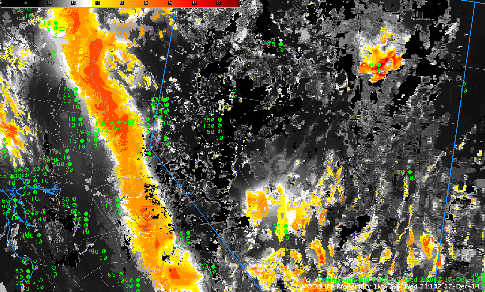
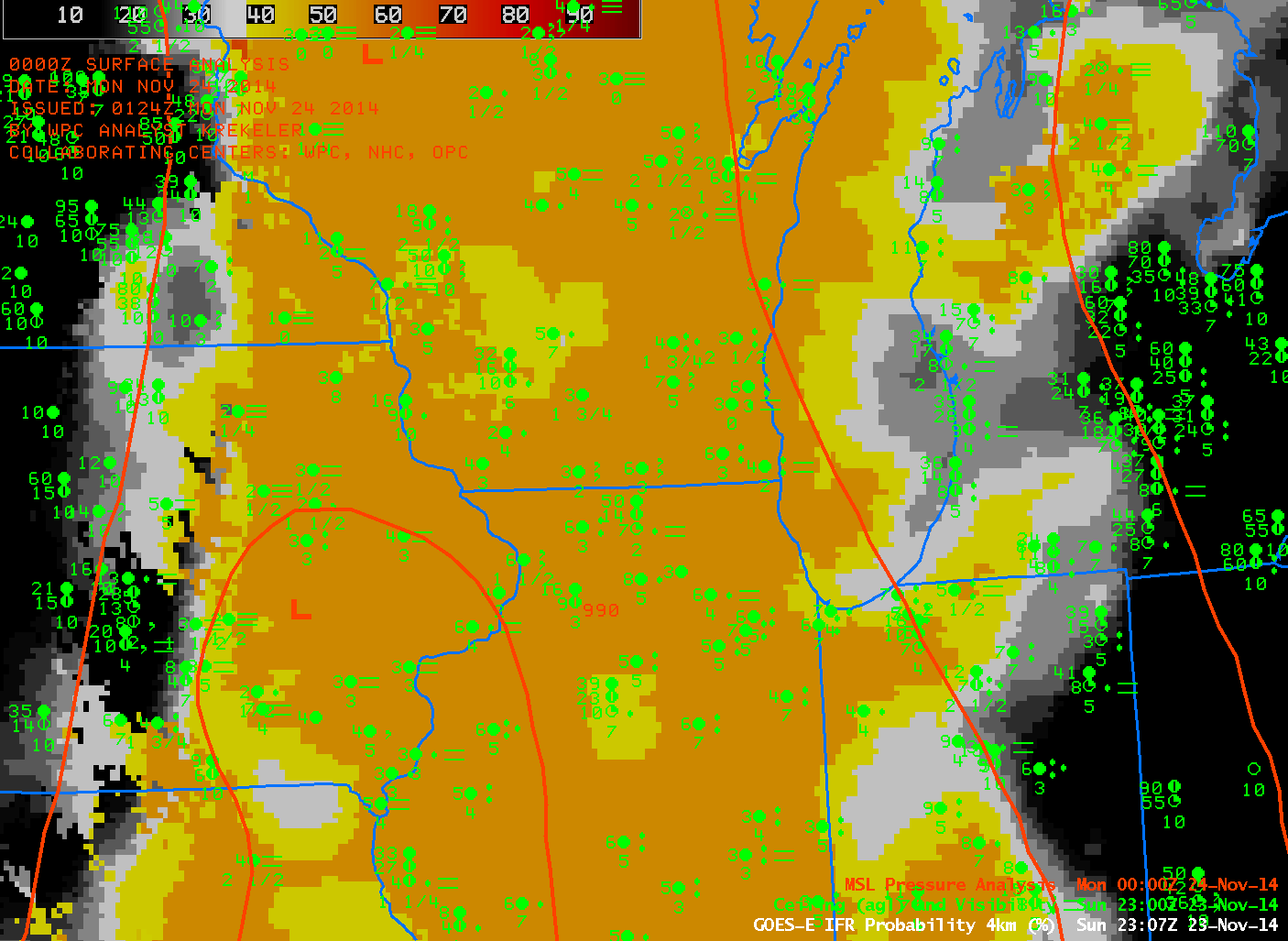
GOES-East-based GOES-R IFR Probabilities and surface-based observations of ceilings and visibilities, hourly from 0145 through 1245 UTC 23 December 2013 (Click to enlarge)

IFR Probability fields show a flat nature that occurs when satellite data cannot be used as a Predictor because of the presence of high clouds/multiple cloud layers. The Probability values are suppressed; interpretation of those values should be colored by the knowledge of the presence or absence of high clouds. In the example above, when high clouds briefly separate over central South Carolina around 0600 UTC, a region of higher IFR probability is shown. The algorithm is more confident that fog/low stratus exists because Satellite Predictors can also be used in that region. What changes is the ability of the GOES-R IFR Probability algorithm to assess the probability of IFR conditions because more predictors can be included; in the region where the high clouds part, satellite information about the low clouds can be included, and IFR Probabilities increase as a result.

IFR Probabilities in High Terrain

GOES-15-based GOES-R IFR Probabilities, hourly from 0000 UTC through 1500 UTC on 18 December 2014 (Click to enlarge)

IFR Probabilities give information about IFR Conditions that occur when terrain ascends up into the clouds, as happens sometimes in the Sierras. A stratus deck might exist over the Central Valley of California, but as that stratus extends to the east, the terrain rises up into the cloud, and IFR conditions result. The animation above shows IFR Probabilities during the night of 17-18 December 2014. Stations at elevation are not common, but Blue Canyon (KBLU) in Placer County is at 1600 meters above sea level. IFR Probabilities in/around north central Placer County (where KBLU is sited) are highest with the visibility is most restricted. Note in the animations that Truckee, CA, to the east of Blue Canyon, does not experience IFR Conditions, perhaps because it is east of the crest of the Sierras.

MODIS data occasionally gives very high-resolution information. The data below from 2100 UTC on 17 December and shows the IFR Probability banked up against the Sierras.

MODIS-based GOES-R IFR Probability, 2113 UTC on 17 December 2014, along with surface-based observations of ceilings and visibilities (Click to Enlarge)

Extended Period of Fog/Low Stratus over the Arizona

GOES-13 Visible Imagery at 1600 and 2300 UTC from 6 December through 13 December 2014 (Click to enlarge)

Northern Arizona experienced a wet start to December (From 2-4 December, Flagstaff received 1.79″, Winslow received 0.80″ and Grand Canyon Airport received 0.41″). When High Pressure and an inversion then settled over the region (an animation of surface weather charts is here), the stage was set for a prolonged period of fog and low stratus, as noted here, for example. The visible imagery, above, testifies to the persistence of the low clouds and fog. It is apparent on 6 December during the day, and persists through the 12th. Visible imagery also shows the presence of high clouds; the presence of those high clouds makes ongoing detection of lower clouds difficult. In addition, both the visible imagery and brightness temperature difference product (10.7 µm – 3.9 µm on GOES-13, historically and still routinely used to detect water-based clouds) give information about the top of the cloud. There is great difficulty in using this information to infer a surface visibility or ceiling (that is, information about the bottom of the cloud).

Fused products have an advantage of incorporating surface-based data (assimilated into the model — the Rapid Refresh in this case) to provide information on whether saturation is occurring in the lowest kilometer of the atmosphere. If that is the case, IFR Probabilities will be larger. The animation below shows Brightness Temperature Difference products and IFR Probabilities at 3 different times (~0700, ~1700 and ~2300) during the days on 8-11 December. IFR Probability fields continually show a strong signal in the region of fog/low stratus over eastern Arizona; the brightness temperature difference field does not, as it is affected by cirrus clouds and by solar reflectivity during the day. Clear skies on 10-11 December at night did allow the brightness temperature difference product to highlight the low clouds over Arizona.

GOES-13 Brightness Temperature Difference (Left, 10.7 µm – 3.9 µm) and IFR Probability (Right) from 8 December through 11 December at ~0700, ~1700 and ~2300 UTC. The Brightness Temperature Difference is enhanced so that fog/low stratus are yellow/orange/red at night, black during the day. (Click to enlarge)

Fog over the Southern Plains

Fog developed over Texas, Oklahoma and Arkansas early in the morning of 9 December 2014. Multiple cloud layers made traditional satellite detection (that is, using brightness temperature difference field (10.7µm – 3.9µm)) problematic. How did the fused product, GOES-R IFR Probability perform? The animation below shows the hourly evolution of IFR Probability from 0215 UTC through 1415 UTC.

GOES-R IFR Probabilities, hourly from 0215 through 1415 UTC on 9 December 2014, along with surface plots of ceilings and visibilities (Click to enlarge)

There are widespread reports of IFR conditions over southeast Oklahoma and northern Texas, as well as over Arkansas in the Arkansas River Valley. IFR Probability fields generally overlap the region of reduced ceilings and visibilities.

Note that the probabilities increased over west Texas between 1315 and 1415 UTC. The boundary between day and night predictors is also apparent at 1415 UTC as a SW to NE line over the Texas Panhandle. Probabilities change as night switches to day because different combinations of satellite predictors can be used. In particular, the use of visible imagery improves cloud clearing and therefore IFR Probabilities increase in regions where low clouds exist (because the possibility of clouds being present is more easily detected).

The toggles below show data from 0615, 1115 and 1415 UTC and demonstrate why a fused product can give better information than a satellite-only product. Intermittent high clouds over the southern Plains prevented GOES-13 from identifying regions of low clouds (Cirrus clouds in the enhancement below appear as dark regions). IFR Probabilities can give valid information in these regions because the Rapid Refresh Model gives information about the possibility of low-level saturation. There are large regions at 1415 UTC over west Texas that are covered by cirrus clouds; despite the inability of the satellite to detect low clouds, IFR Probability maintains a strong signal there where IFR Conditions are occurring. The 1415 Brightness Temperature Difference field, in contrast to the IFR Probability field, gives very little information because increasing amounts of solar radiation are changing the relationship between 10.7µm and 3.9µm radiation at 1415 UTC.

GOES-R IFR Probabilities and GOES-13 Brightness Temperature Difference Fields (10.7µm – 3.9µm), 0615 UTC on 9 December 2014, along with surface observations of ceilings and visibilities (Click to enlarge)

As above, but at 1115 UTC (Click to enlarge)

As above, but at 1415 UTC (Click to enlarge)

A near-Full Moon on 9 December means that the Day Night Visible imagery from Suomi NPP produced great imagery of the clouds over the southern Plains. The toggle below shows the Day Night band, the brightness temperaure difference field (11.35µm – 3.74µm) and the topography. Very narrow fog banks are apparent over southeast Oklahoma and over Arkansas, nestled into narrow valleys. The Brightness Temperature Difference field distinguishes between water-based clouds (presumably low stratus or fog) in orange and ice clouds (cirrus) in black.

Suomi NPP Brightness Temperature Difference (11.35µm – 3.74µm) fields, Day Night band imagery and Color-shaded topography, 0839 UTC 9 December 2014 (Click to enlarge)

The fog event over Dallas was photographed from the air: Link.

More fog over South Carolina

Dense fog redeveloped over South Carolina overnight on 3-4 December 2014, and as noted in the Forecast Discussion below, its character was just a bit different than on the previous night.

000
FXUS62 KCHS 040239
AFDCHS

AREA FORECAST DISCUSSION
NATIONAL WEATHER SERVICE CHARLESTON SC
939 PM EST WED DEC 3 2014

.SYNOPSIS…
UNDER A WEAKENING WEDGE OF HIGH PRESSURE…FOG WILL PERSIST TONIGHT.
ANOTHER AREA OF HIGH PRESSURE WILL BUILD FROM THE NORTH THURSDAY THROUGH
FRIDAY. A WARM FRONT WILL THEN LIFT ACROSS THE AREA ON SATURDAY…
BEFORE A COLD FRONT MOVES THROUGH SATURDAY NIGHT. AN INLAND WEDGE
OF HIGH PRESSURE WILL BECOME ESTABLISHED SUNDAY AND MONDAY…FOLLOWED
BY THE PASSAGE OF ANOTHER COLD FRONT MONDAY NIGHT. HIGH PRESSURE
WILL THEN PREVAIL INTO THE MIDDLE OF NEXT WEEK.

.NEAR TERM /UNTIL 6 AM THURSDAY MORNING/…
WHILE THE SCENARIO IS QUITE DIFFERENT FOR FOG TONIGHT COMPARED TO
LAST NIGHT…DESPITE PLENTY OF CIRRIFORM CLOUDS /SOME OF WHICH ARE
OPAQUE/…WE ARE STILL GETTING AREAS OF FOG TO FORM. SOME OF THE
FOG IS ALREADY DENSE…ESPECIALLY IN THE CHARLESTON QUAD COUNTY
AREA AND ALONG OUR COASTAL ZONES SOUTH INTO MCINTOSH. THIS IS A
MIX OF STRATUS BUILD-DOWN AND ADVECTIVE FOG FROM OFF THE ATLANTIC.
SO WE LOOK FOR A FURTHER EXPANSION OF THE FOG INLAND TO THE WEST
OF I-95 THROUGH THE NIGHT. DENSE FOG ADVISORIES WILL THEREFORE
REMAIN IN EFFECT.

GOES-based GOES-R IFR Probabilities, hourly from 2315 UTC 3 December through 1015 UTC on 4 December as well as observations of ceilings (AGL) and visibilities (Click to enlarge)

GOES-R IFR Probabilities, above, (click here for an animation with a faster dwell rate) once again capably outlined the region of IFR conditions over South Carolina. Probabilities are lower when Satellite data cannot be used as a predictor, as when cirrus clouds prevent the satellite from viewing water-based clouds closer to the surface. In such cases when only Rapid Refresh model data can be used as Fog Predictors, the fields take on a flatter, less pixelated character as above. There are a few regions where breaks in the cirrus cloud allow Satellite predictors to be incorporated in the IFR Probability fields, for example along the South Carolina coast at 0600 UTC. When high clouds are present, interpret the magnitude of the IFR Probability in a different way than when high clouds are absent. An IFR Probability of 55% in a region of cirrus clouds has a different meaning than an IFR Probability of 55% in a region of only low clouds.

Because of Cirrus clouds, the brightness temperature difference fields gave almost no information about the presence of low clouds. See the animation below (a loop with a faster dwell rate is here).

GOES-13 Brightness Temperature Difference Fields (10.7µm – 3.9µm), hourly from 2315 UTC 3 December through 1015 UTC on 4 December, as well as observations of ceilings (AGL) and visibilities (Click to enlarge)

Dense Fog over South Carolina

Dense fog devloped over South Carolina overnight, in an event that was well-anticipated: From the Charleston, SC, National Weather Service Office AFD (emphasis added):

AREA FORECAST DISCUSSION
NATIONAL WEATHER SERVICE CHARLESTON SC
648 PM EST TUE DEC 2 2014

.SYNOPSIS…
WEAK HIGH PRESSURE WILL PERSIST THROUGH WEDNESDAY. A COLD FRONT
WILL ADVANCE SOUTH THROUGH THE AREA THURSDAY…THEN HIGH PRESSURE
WILL BUILD FROM THE NORTH AND WILL PREVAIL THROUGH FRIDAY. LOW
PRESSURE WILL TRACK THROUGH OR JUST NORTH OF THE REGION SATURDAY…
FOLLOWED BY COLD FRONTS SATURDAY NIGHT AND AGAIN LATE MONDAY.

.NEAR TERM /UNTIL 6 AM WEDNESDAY MORNING/…
A FEW LINGERING STRAY SHOWERS WEST OF I-95 WILL DISSIPATE THIS
EVENING WITH THE ONSET OF NOCTURNAL COOLING AND STABILIZATION.

OUR MAIN FOCUS FOR TONIGHT IS IN REGARDS TO FOG AND THE BUILD DOWN
OF STRATUS…SOME OF WHICH COULD BE DENSE. THE HIGH PRESSURE WEDGE
WILL REMAIN ANCHORED OVER THE INLAND PARTS OF THE SE AS IT
PROGRESSES A LITTLE SOUTHWARD THROUGH THE NIGHT…WITH A WEAK
COASTAL TROUGH OFFSHORE. A STRENGTHENING NOCTURNAL INVERSION WILL
DEVELOP AND TRAP ABUNDANT MOISTURE WITHIN THE PLANETARY BOUNDARY
LAYER UNDERNEATH. THIS WILL LEAD TO THE DEVELOPMENT AND SPREADING
OUT OF FOG AND STRATUS ENCOMPASSING MOST IF NOT ALL OF THE CWFA
DURING THE LATE NIGHT HOURS. BUT ALREADY WE/RE SEEING A FOG BANK
WITH IT/S ORIGINS NORTH OF THE SANTEE RIVER THIS AFTERNOON IS
PROGRESSING SOUTH/SW AND STARTING TO SPREAD A LITTLE INLAND. THIS
IS CLEARLY DEPICTED BY THE 11-3.9 MICRON SATELLITE IMAGERY AS WELL
AS COASTAL METAR SITES. THE COMBINATION OF THE MARINE INDUCED FOG
AND STRATUS WILL COMBINE WITH RADIATION FOG THAT FORMS OVER INLAND
SECTIONS TO RESULT IN AREAS OF FOG ACROSS THE FORECAST ZONES. THE
WORST CONDITIONS WILL BE OVER CHARLESTON COUNTY THIS
EVENING…SPREADING INTO OTHER COASTAL SC ZONES LATER THIS EVENING
AND INTO THE GA COASTAL ZONES BY MIDNIGHT OR SO. INLAND THE BULK
OF THE GREATER FOG/STRATUS COVERAGE WILL WAIT UNTIL WE REACH OUR
CROSS-OVER TEMPS BY 2-3 AM. DENSE FOG ADVISORIES ARE CERTAINLY
POSSIBLE. ANY NEGATING FACTORS AGAINST THE WIDESPREAD DENSE FOG
WOULD BE THE RELATIVELY WARM GROUNDS. BUT GIVEN FOG STABILITY
INDICES IN THE TEENS AND LOWER 20S…MOST PLACES REACHING THEIR
CROSS-OVER TEMPS OF 55-60 AND SOME MARINE FOG WE/D LEAN MORE
TOWARD DENSE FOG BECOMING A CONCERN…THAN NOT.

GOES-based GOES-R IFR Probabilities, hourly from 2215 UTC 2 December through 1315 UTC on 3 December as well as observations of ceilings (AGL) and visibilities (Click to enlarge)

The GOES-R IFR Probability fields, shown at hourly intervals above, nicely capture the spread of the extensive fog as the expanding marine fog bank joins up with the developing radiation fog over northwestern South Carolina. (A loop with a shorter dwell rate is here). GOES-13 Brightness Temperature Difference Fields are shown below. (A loop with a shorter dwell rate is here). Brightness Temperature Difference is the traditional method of detecting fog and low stratus, and it is referenced in the AFD above. However, the method cannot operate in regions with high cirrus (such as over Tennessee and northwest South Carolina after 0900 UTC); the brightness temperature difference signal flips sign as the sun rises (as at 1315 UTC in the animation below); the method cannot distinguish between elevated stratus and visibility-restricting fog.

GOES-13 Brightness Temperature Difference Fields (10.7µm – 3.9µm), hourly from 2215 UTC 2 December through 1315 UTC on 3 December, as well as observations of ceilings (AGL) and visibilities (Click to enlarge)

In comparing the two animations, note how the Brightness Temperature Difference field, for example, has strong returns around 0215-0315 UTC over central South Carolina in regions where widespread IFR conditions do not yet exist. In these regions, the Rapid Refresh model data used as a predictor in the GOES-R IFR Probability is not yet showing saturation, so IFR Probabilities aren’t quite so high as they are along the coast. (Click here for a toggle between the GOES-R IFR Probability and the Brightness Temperature Difference fields at 0215 UTC; a toggle at 0315 UTC is here). Note also in the toggles how the IFR Probability fields have little signal over Georgia despite the Brightness Temperature Difference field signal. This demonstrates the power of using fused data products: both the satellite and the model signal must be in accord for very high probabilities to occur.

Ice Fog causes Flight Diversions at Denver International

Ice Fog at Denver International Airport on Sunday 30 November resulted in the diversion of almost 50 flights. (News Link) From the link:

Sunday morning fog caused about 46 flights scheduled to land at Denver International Airport to be diverted, airport officials said.

GOES-R IFR Probability Fields, every 15 minutes, from 0500 UTC through 2200 UTC on 30 November 2014, along with surface reports of ceilings and visibility (Click to enlarge)

The GOES-R IFR Probability field gave useful anticipatory information for this event. The animation above shows a line of high IFR Probability moving southward and westward. Stations within the highest IFR Probability reported freezing fog (e.g. Sidney Nebraska (KSNY) at 0800 UTC, Akron, CO (KAKO) at 1200, 1300 and 1400 UTC and Kit Carson Airport in Burlington CO (KITR) at 1400 UTC). When the region of higher IFR Probability abuts up against Denver International (KDEN), then, at 1600 UTC, the Freezing Fog that occurred should not surprise. This region of enhanced IFR Probability persisted near Denver International through 2200 UTC.

The METARS, listed below, show the onset of the freezing fog (FZFG). Note that times are boldface in black, and fog-related observations are boldfaced in red:

KDEN 301353Z 13005KT 10SM FEW110 BKN220 07/M13 A2981 RMK AO2
SLP068 T00721128 $=
KDEN 301453Z 17007KT 10SM FEW110 SCT220 06/M11 A2984 RMK AO2
SLP082 FG BANK DSNT NW-SE T00561111 51034 $=
KDEN 301539Z 07016KT 1/2SM R35L/P6000FT FZFG FEW001 FEW110
SCT220 M06/M08 A2988 RMK AO2 WSHFT 1505 FG FEW001
T10611078 $=
KDEN 301542Z 07017KT 1/4SM R35L/P6000FT FZFG FEW001 FEW110
SCT220 M06/M07 A2989 RMK AO2 WSHFT 1505 FG FEW001 VIS W
1/2 T10611072 $=
KDEN 301553Z 07019KT 1/4SM R35L/2200VP6000FT FZFG VV002
M06/M07 A2991 RMK AO2 WSHFT 1505 PRESRR SLP131 FROPA
I1000 T10611072 $=
KDEN 301630Z 07020KT 1/8SM R35L/1400V2200FT FZFG VV001
M06/M07 A2993=
KDEN 301637Z 08019KT 1/4SM R35L/1400V2400FT FZFG VV001
M06/M07 A2994 RMK AO2 PK WND 07026/1633 TWR VIS 1/4
I1004 T10611072 $=
KDEN 301651Z 08021G28KT 1/4SM R35L/1000V1600FT FZFG VV002
M07/M07 A2995 RMK AO2 PK WND 07028/1643 I1004 $=
KDEN 301653Z 08023KT 1/4SM R35L/1000V1400FT FZFG VV002
M07/M07 A2996 RMK AO2 PK WND 07028/1643 SLP145 I1004
T10671072 $=

(Click here to see a more English Language Listing; Click here to see a meteorogram)

GOES-13 Brightness Temperature Difference fields (10.7µm – 3.9µm) from 0800 through 1600 UTC on 30 November 2014 (Click to enlarge)

For comparison, the Brightness Temperature Difference Field is shown above. Terrain-induced cirrus clouds largely obscured the view of low clouds from satellite in this case. Thus, the incorporation of surface information via the Rapid Refresh model was key to producing an IFR Probability field with useful content.

Visible Imagery from GOES-13 (below) and GOES-15 (bottom) show the cirrus and the underlying low clouds. The steady southward advancement of the low clouds is consistent with the motion of the IFR Probability fields.

GOES-13 Visible Imagery (0.63µm) animation, 1400-1800 UTC on 30 November 2014 (Click to enlarge)

GOES-15 Visible Imagery (0.62µm) animation, 1400-1800 UTC on 30 November 2014 (Click to enlarge)

Advection Fog with a Cyclone over the Midwest

GOES-based GOES-R IFR Probabilities and surface observations of Ceilings and Visibilities, ~2300 UTC, and the 0000 UTC HPC Analysis of surface pressure (Click to Enlarge)

In the image above, a trough of low pressure is depicted along the Mississippi River, with moist southerly flow over the Ohio Valley and Western Great Lakes (Dewpoints in Wisconsin at this time were mid- to upper-40s (Fahrenheit). This moist air is easily cooled to its dewpoint by the underlying cool ground, and dense fog is a result. However, this fog is difficult to detect from satellite because of the multiple cloud layers that accompany low pressure systems. GOES-R IFR Probabilities show a good signal because of Fog Predictors that are derived from numerical model output (the numerical model used is the Rapid Refresh). In this case, the Rapid Refresh was accurately depicting the evolution of the system because the model-based field of IFR Probabilities accurately overlaps the region of observed IFR (and near-IFR) conditions.

Fused Products yield better Output

GOES_IFR_US_11-3.9_Sat_20141121_1100toggle

GOES-R IFR Probabilities computed from GOES-East, and GOES-East Brightness Temperature Differences (10.7 µm – 3.9 µm), 1100 UTC on 21 Nov 2014 (Click to enlarge)

The traditional method of detecting fog/low stratus from satellite data, the brightness temperature difference between the longwave and shortwave infrared channels (10.7 µm – 3.9 µm on GOES) can overpredict regions of reduced ceilings and visibilities because satellites see only the top of the cloud. GOES-R IFR Probabilities, in contrast, incorporate surface-based information into a fog/low stratus predictive algorithm. As a result, regions with elevated stratus (such as eastern/northeastern Oklahoma in the toggle above) that should not affect transportation (for example) can be screened out of a field meant to diagnose regions of reduced visibilities.

Low Ceilings/visibilities over the Deep South in the wake of a cold frontal passage

GOES-R IFR Probabilities ~hourly from 0200-1215 UTC on 17 November along with surface plots of ceilings and visibilities (Click to enlarge)

A strong cold front moved through the deep south in the early morning of 17 November 2014, accompanied by low ceilings and reduced visibilities that were very close to IFR conditions. Multiple cloud layers, however, prevented brightness temperature difference fields from diagnosing the low clouds. In cases such as these, a data fusion product such as GOES-R IFR Probability that incorporates surface information via a model simulation (such as the Rapid Refresh) that assimilates surface data is still able to highlight regions where IFR Conditions are most likely. In the animation above, flat fields (those that are horizontally homogeneous, such as over central Mississippi at 0315 UTC) are regions where multiple cloud layers prevent the identification of low cloud features and GOES-R IFR Probability is therefore computed using model-based predictors only. Regions over Louisiana at the beginning of the animation are more pixelated in appearance. This is a region where high clouds have pushed off to the East, where satellites can observe the behavior of low stratus and where satellite data can therefore be used as a predictor in the GOES-R IFR Probability algorithm. Regions where satellite data cannot be used generally have lower probabilities because one of the predictors (satellite data) is absent. That is the case in the above animation. When satellite data can be used, IFR Probabilities increase. Use that knowledge of the behavior of IFR Probability fields to tailor your interpretation of the magnitude of the IFR Probability.

GOES-R Fog Product Examples

Fog detection fusing GOES, Terra/Aqua or Suomi/NPP Satellite data with Model output