GOES_16 Visible imagery, above (along with surface observations of ceilings and visibilities), shows fog and low clouds over south Texas and offshore waters. The observations plotted can allow you to determine where IFR conditions are apparent — where visibilities are between 1 and 3 statute miles and ceilings are between 500 and 1000 feet. It’s difficult to determine the area of IFR conditions based solely on cloud cover however.
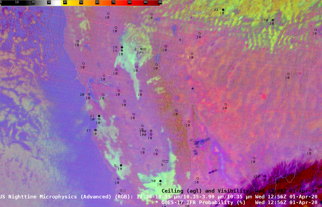
The animation below shows the probability of IFR conditions, a product that fuses satellite information with low-level saturation information from the Rapid Refresh model (Click here for an animation with no observations). The morning fog over east Texas burns off fairly quickly, and only dense sea fog is left after about 1700 UTC (10 AM CDT). In many offshore regions (and over east Texas before sunrise), the IFR Probability field has a flat character to it that is typical of a IFR Probability field determined mostly by model data. More pixelated data (and somewhat higher probabilities) occur where breaks in the cloud allow for satellite data to identify low clouds.
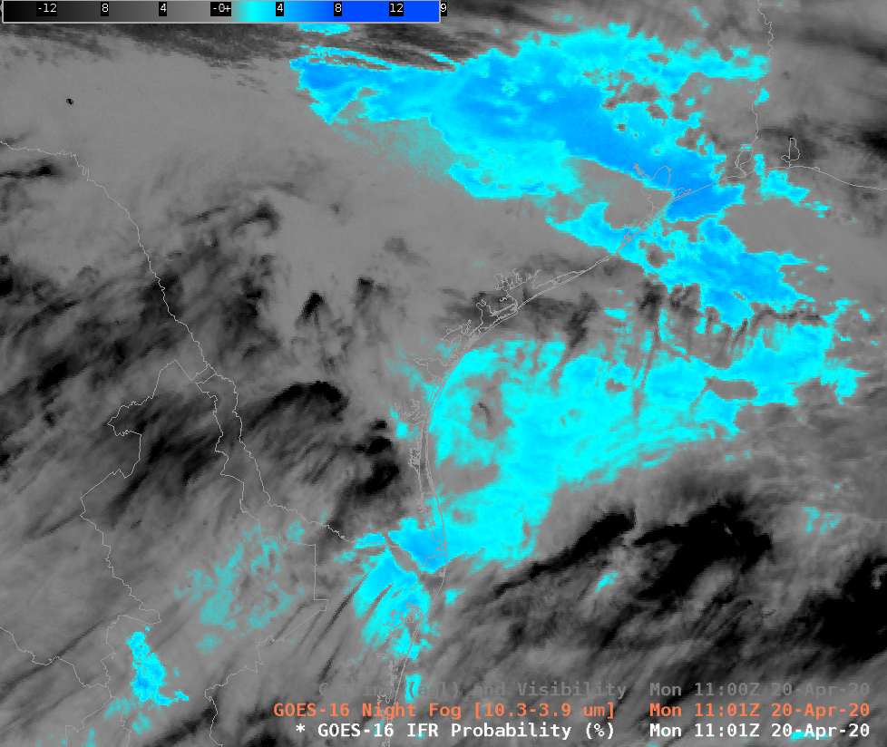
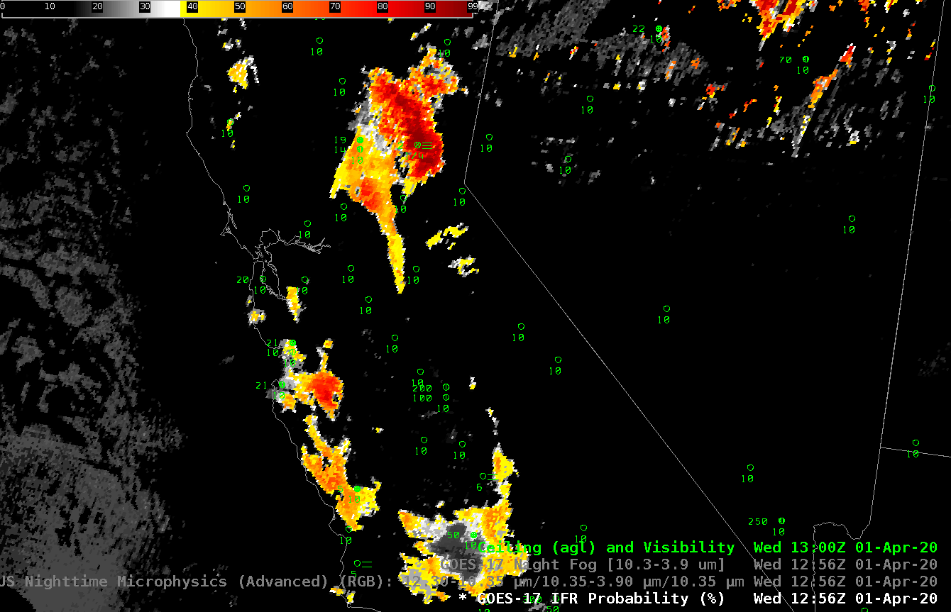
The night fog brightness temperature difference field, below, highlights a challenge in identifying low clouds using satellite data alone (in contrast to the IFR Probability above that uses satellite and model data, fusing the strengths of both). When cirrus is present, it can mask the satellite’s view of the low cloud beneath. In addition, the Night Fog Brightness Temperature difference product is not consistent through sunrise, as the emissivity differences that drive the signal at night time (small cloud droplets are not black body emitters of 3.9 µm radiation, but they are blackbody emitters of 10.3 µm radiation) become overwhelmed by reflectivity differences during the day when far more 3.9 µm solar radiation is reflected than 10.3 µm solar radiation. Thus, in the day, both low clouds and high clouds show up as black in this enhancement: they are both able reflectors of 3.9 µm radiation.

The Day Fog Brightness Temperature Difference field, below, shows how cirrus ice crystals are initially more reflective of solar radiation, but as the sun climbs higher in the sky, low clouds start to reflect just as much solar radiation.
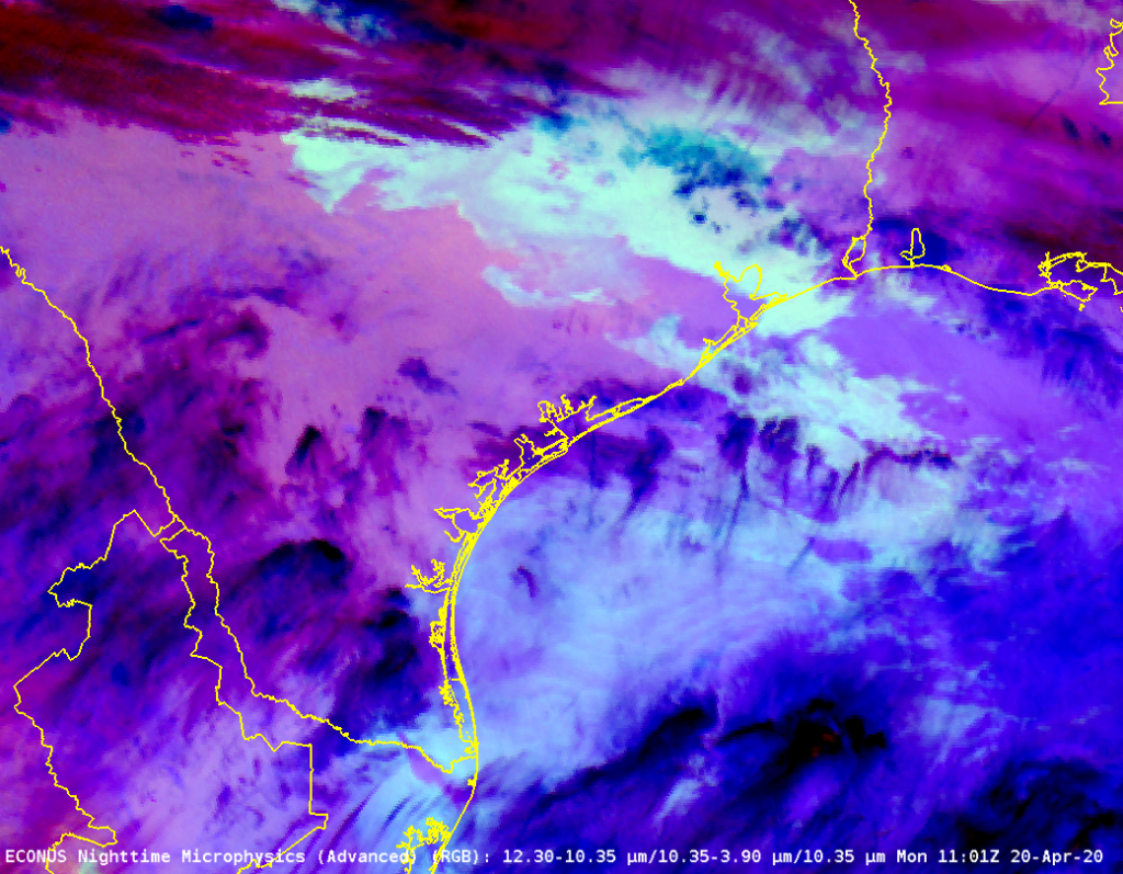
The Night Fog Brightness Temperature Difference field, above, is a key component (the ‘green’ part) of the Advanced Night Time Microphysics RGB, shown below. Where the Brightness Temperature Difference field is unable to view low clouds, similarly the Night Time Microphysics RGB will be unable to highlight them.
Thanks to Penny Harness, WFO Corpus Christi, for alerting us to this event. (Link)
