Monthly Archives: January 2017

Ice Fog in Kansas City

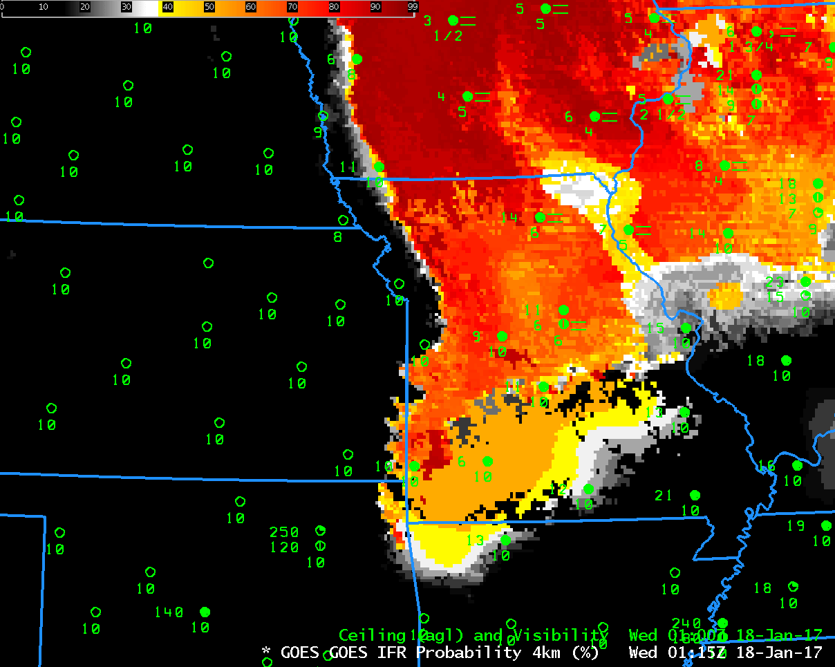
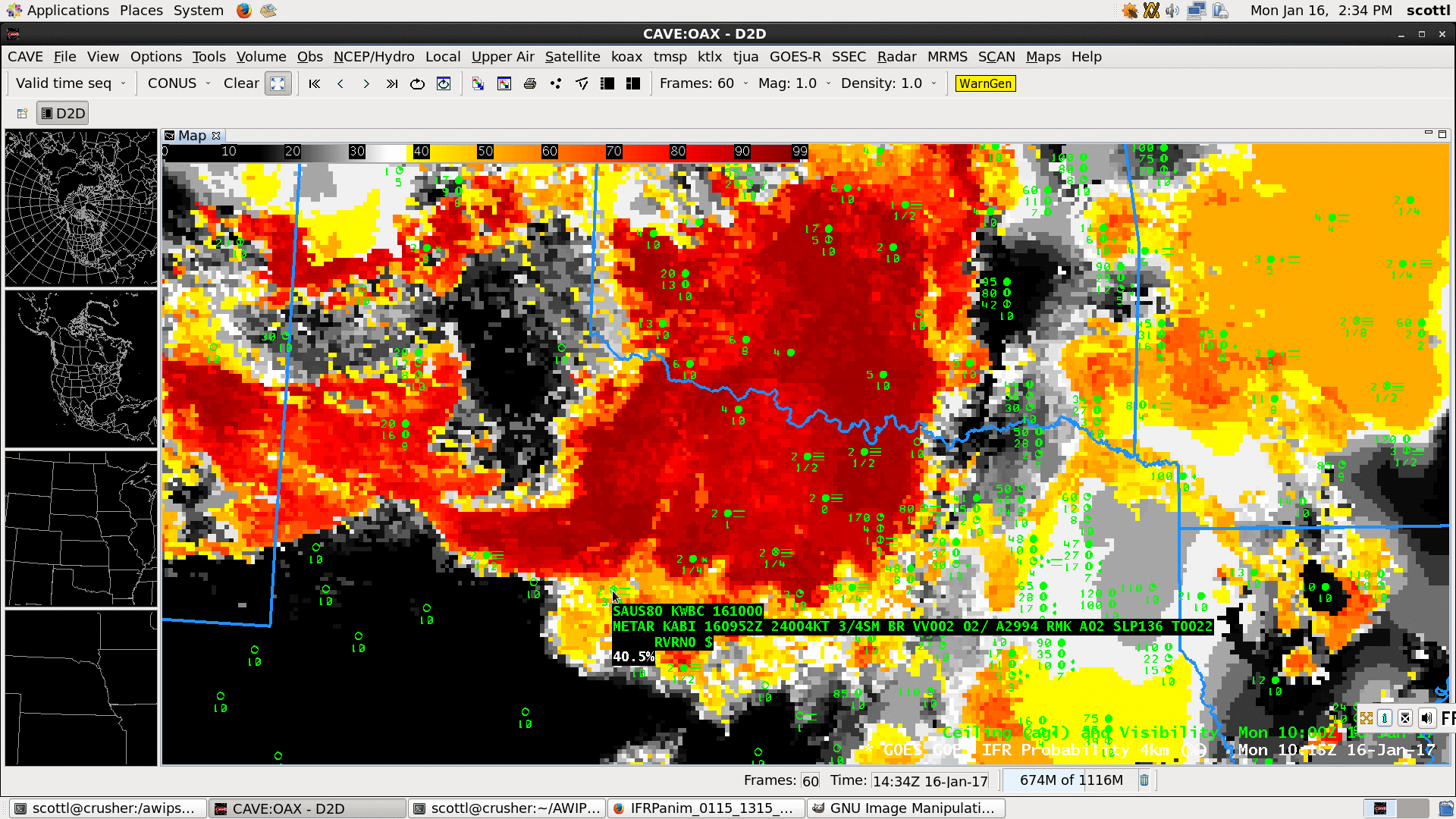
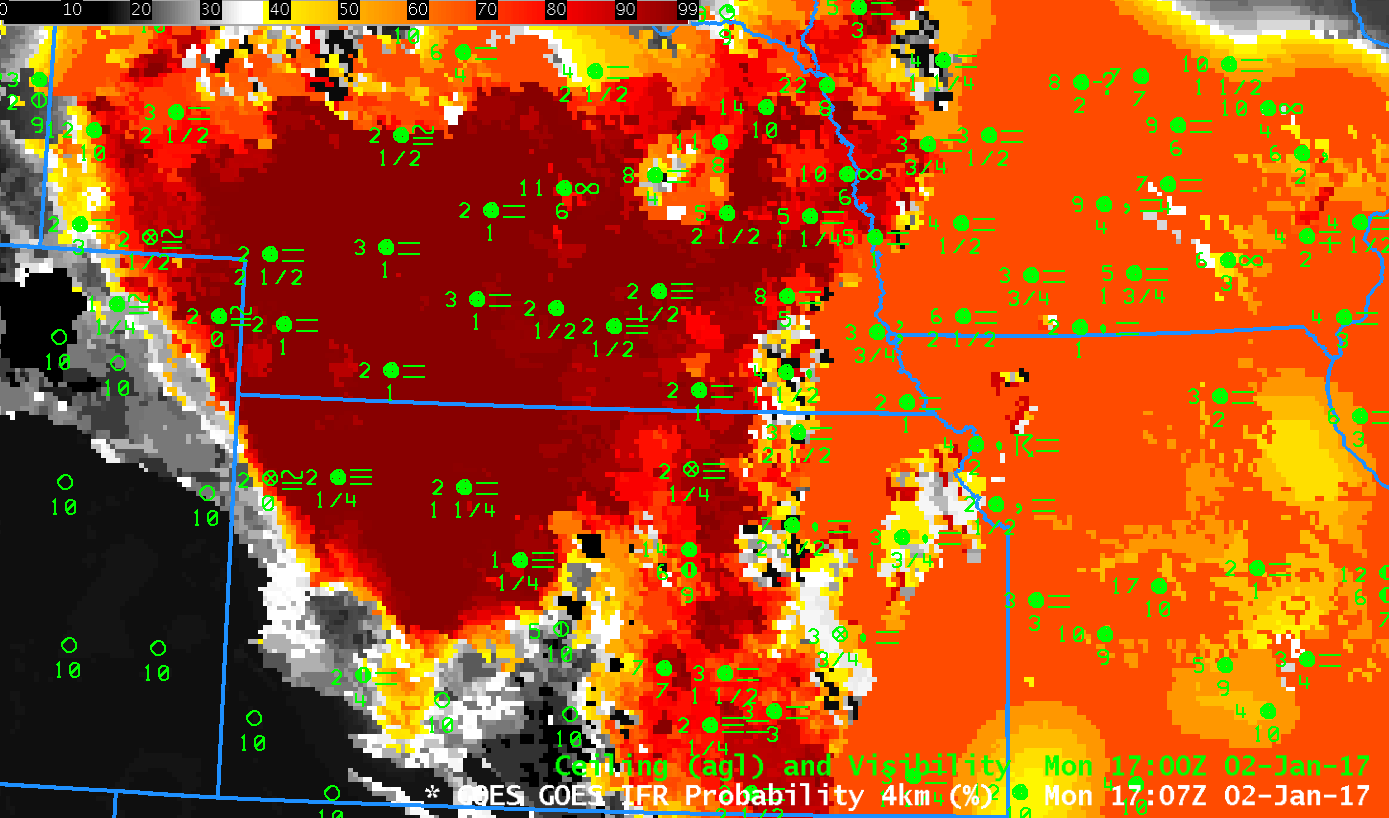
GOES-R IFR Probabilities, hourly from 0115 through 1815 UTC, and surface observations of ceilings and visibilities, on 18 January 2017 (Click to enlarge)

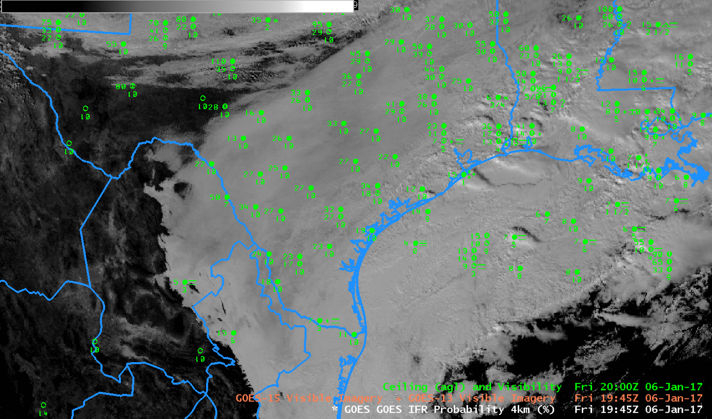
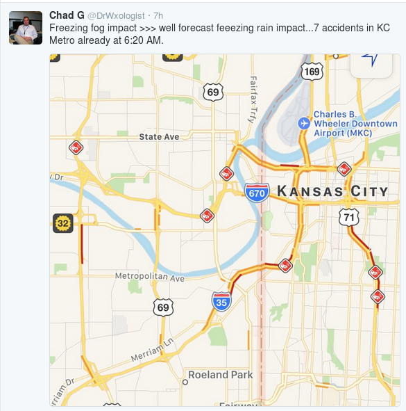
Ice Fog developed over Kansas City during the early morning hours of 18 January 2017, with accidents that snarled traffic (tweeted image courtesy @DrWxologist Chad Gravelle)  starting before sunrise and continuing through the morning rush hour  (Screenshot of News link from here).    Dense Fog Advisories were issued.  The animation above, of GOES-R IFR Probability fields, shows the slow westward progression of the Fog/Low Clouds into the Kansas City Metro area shortly after 4 AM CST.  High IFR Probabilities persist through 1800 UTC and diminished shortly thereafter.

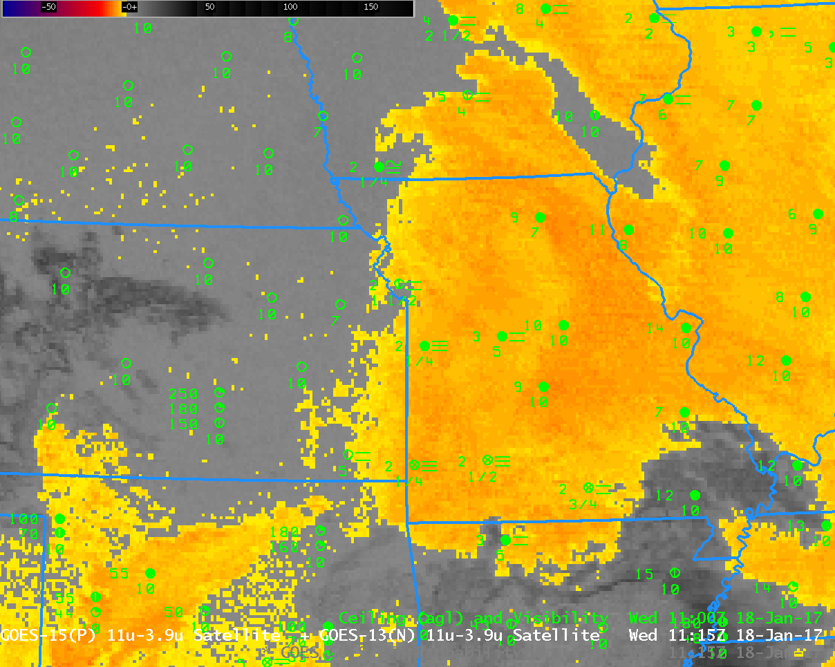
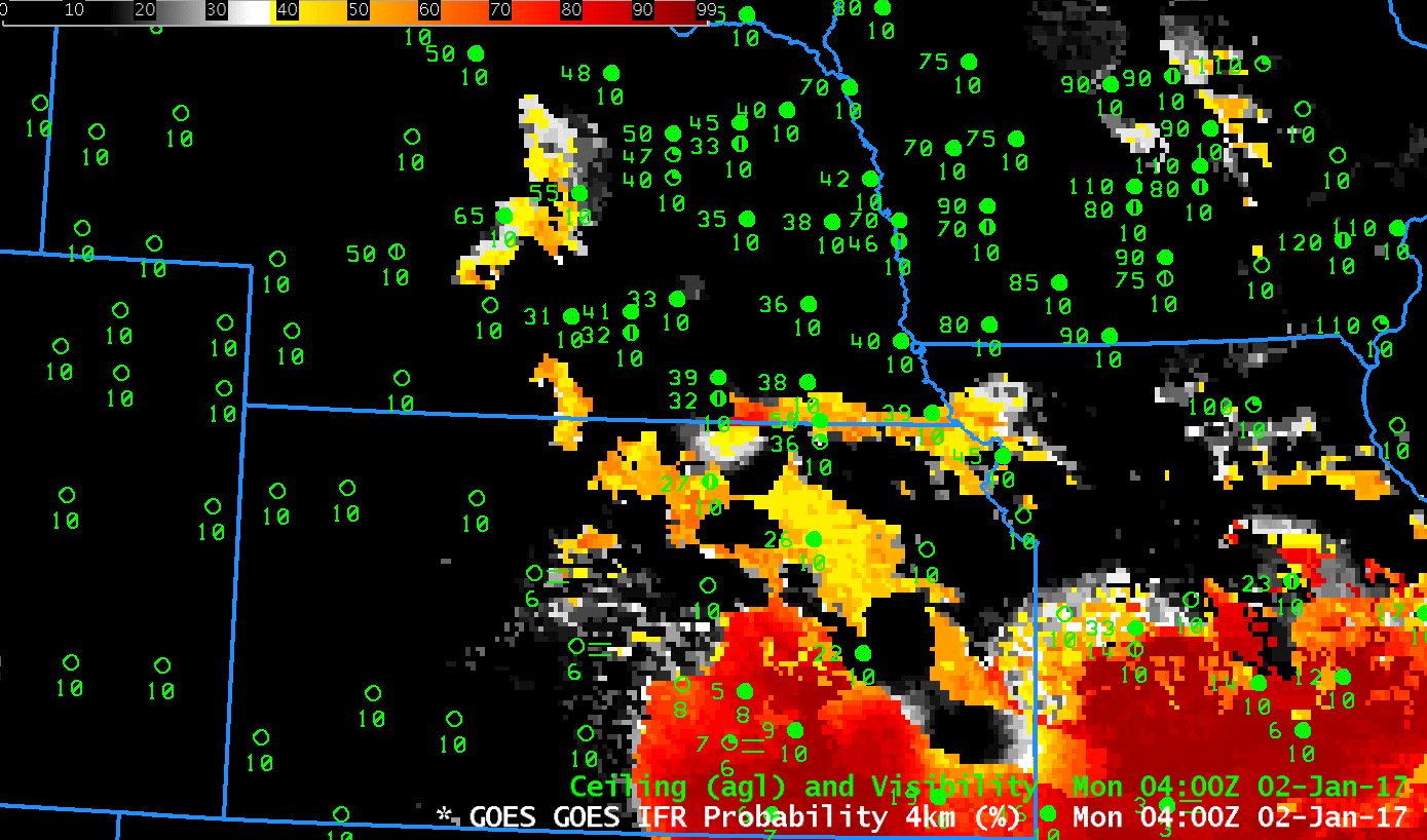
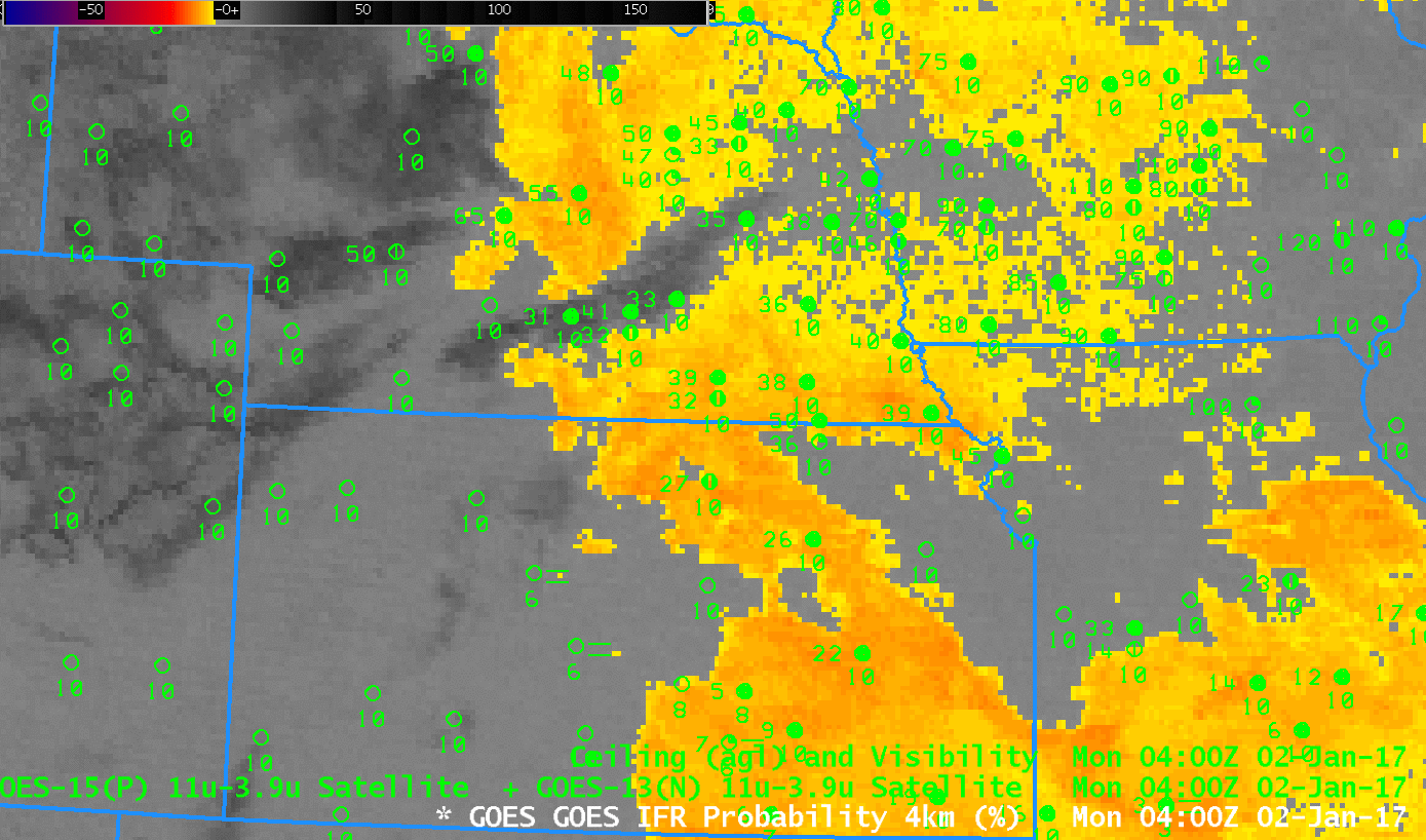
During this case, an absence of mid-level and high clouds allowed IFR Probabilities to reach very large values.  The toggle below shows Brightness Temperature Difference fields (3.9 – 10.7) and GOES-R IFR Probabilities at 1115 UTC.  Low clouds cover Missouri except for the region over the Missouri Bootheel.  Note that the western edge of the satellite-detected low clouds is slightly to the east of the western edge of the IFR Probability in this case.  Model data are suggesting that low-level saturation is occurring in those regions (over far southwest Iowa, for example) although satellite data were not yet showing a strong signal.  Observations show IFR conditions (at Clarinda, Iowa, for example, where freezing fog is reported with 200-foot ceilings and 1/4-mile visibility).

Dense Fog over the Carolinas

GOES-13 Brightness Temperature Difference (3.9 µm – 10.7 µm), GOES-R IFR Probability and GOES-R Cloud Thickness at 1115 UTC on 17 January 2017 (Click the enlarge)

Dense Fog Advisories (National Weather Service Website) and IFR SIGMETs (Aviation Weather website) were issued early in the morning for dense fog over the southeastern United States.  The toggle above from 1115 UTC on 17 January shows the Brightness Temperature Difference field (3.9 µm – 10.7 µm), the GOES-R IFR Probability Field, and the GOES-R Cloud Thickness fields associated with this dense fog event.  Note the presence of high clouds over northern South Carolina and western North Carolina — the dark region in the Brightness Temperature Difference enhancement — prevents the brightness temperature difference field from highlighting that region of reduced ceilings/visibilities.  The GOES-R Cloud Thickness field is not computed under cirrus either, as it relates 3.9 µm emissivity of water-based clouds to cloud thickness (based on a look-up table generated using data from a SODAR off the West Coast of the United States).  If cirrus blocks the view, then, neither the Brightness Temperature Difference field nor the GOES-R Cloud Thickness field can give useful information about low clouds.

In contrast, the GOES-R IFR Probability field does give useful information in regions where cirrus clouds (and low clouds/fog) are present — because Rapid Refresh information about the lower troposphere can be used.  IFR Probability values will be smaller in those regions because satellite predictors are unavailable, and the Probability incorporates both predictors from satellites and from Rapid Refresh model output — if the satellite predictors are missing because of cirrus, the IFR Probability values will be affected. Despite the smaller values, however, the IFR Probability fields in regions of cirrus are giving useful information for this event.

GOES-R Cloud thickness fields can be used to estimate Fog dissipation using the last GOES-R Cloud Thickness field produced before twilight conditions at sunrise (shown below for this case). (GOES-R Cloud Thickness is not computed during twilight conditions because of rapidly changing 3.9 µm emissivity related to the reflected solar radiation as the sun rises, or as it sets). This scatterplot gives the relationship between thickness and dissipation time after the Cloud Thickness time stamp (1215 UTC in this case).  In this case, the thickest fog is near Athens GA;  the algorithm predicts that clearing should happen there last, at about 1515 UTC.

GOES-R Cloud Thickness, 1215 UTC on 17 January 2017 (Click to enlarge)

Widespread IFR Conditions over the Plains

GOES-R IFR Probability Fields, hourly from 0115-1315 UTC (Click to enlarge)

A cyclone over the southern Plains, in addition to causing severe weather over Texas on 15 January also generated widespread IFR Conditions over the southern Plains, as shown below in screengrabs from the Aviation Weather Center and from the National Weather Service. An overnight Water Vapor image (here) testifies to the ubiquitous presence of high clouds over the Plains; in such cases with widespread high clouds, low-cloud detection by satellite is a big problem. A strength of the GOES-R IFR Probability field is that it is a fused data product, incorporating both satellite information (not particularly useful for much of the overnight hours on 15-16 January) and Rapid Refresh model data that can be used to discern conditions near the surface. When the Rapid Refresh model suggests saturation is occurring near the surface (in, say, the lowest 1000 feet of the model atmosphere), IFR Probabilities will be large. They won’t be as large as they might be if both satellite and model data suggest low clouds are present, but useful information emerges in the IFR Probability fields, above, where the Rapid Refresh is predicting low-level saturation. IFR Probabilities are large over much of the southern Plains where IFR conditions are observed. This is the region where the color enhancement is orange.

The low pressure system develops such that high clouds diminish over Texas and Oklahoma. When that happens, the IFR Probability fields change in two ways. First, values increase because satellite data and model data can be used as predictors. When only model data can be used, IFR Probability fields will have smaller values. Secondly, the character of the IFR Probability field takes on a more pixelated appearance because the satellite data values will vary from pixel to pixel. In contrast, when only model data can drive the IFR Probability field (for example, over Kansas at the beginning of the animation), the IFR Probability fields vary quite slowly from pixel to pixel in part because of model smoothing.

Screen Capture from Aviation Weather Center (left, showing widespread IFR Conditions) and from Weather.Gov (right, showing Dense Fog Advisories in grey) (Click to enlarge)

The toggle below includes sampling over Abilene, TX (KABI), a station at the edge of the IFR Probability field. IFR Probabilities are relatively constant at ~40% for the two hours shown, but station conditions change from IFR to VFR. IFR Probabilities at Abilene become quite small by 1315 UTC, at the end of the animation above.

GOES-R IFR Probability at 1015 and 1215 UTC on 16 January 2017. Station conditions at KABI are indicated by the sample probe (Click to enlarge)

Stratus over Texas

GOES-13 Visible (0.64 µm) Imagery, 1945 UTC on 6 January 2017 and surface observations of ceilings and visibilities (click to enlarge)

Visible imagery over Texas shows an extensive stratus deck blanketing the southern and eastern portions of the state.  Can you tell at a glance — without looking at the observations — if the stratus is extending to the surface?  The animation below shows how GOES-R IFR Probabilities describe the scene, with highest IFR Probabilities offshore (where dense fog is observed over the warm water).  Higher Probabilities also hug the high terrain of eastern Mexico, where IFR conditions are also reported (at Monclova, ID MMMV, where a 500-foot ceiling and 3-mile visibility is reported).  The toggle below cycles through the visible and GOES-R IFR Probability fields and also includes terrain.

GOES-R IFR Probability provides useful situational awareness information during the daytime as well as at night.

GOES-13 Visible (0.64 µm) Imagery, 1945 UTC on 6 January 2017 and surface observations of ceilings and visibilities, and with surface analysis superimposed, as well as GOES-R IFR Probabilities (1945 UTC) and Terrain (click to enlarge)

Persistent IFR Conditions over Kansas

GOES-R IFR Probability fields, 0400-1700 UTC on 2 January 2017 (Click to enlarge)

Late in the morning on Monday 2 January 2017, the weather.gov website shows Dense Fog Advisories persisting in parts of Kansas and Nebraska.  The animation above shows GOES-R IFR Probabilities from 0400 through 1700 UTC on the 2nd. High IFR Probabilities show excellent correspondence with very low ceilings and reduced visibilities. Note, for example, the sharp demarcation at 1700 UTC between IFR conditions (and large IFR Probabilities) and VFR/MVFR conditions (and very low IFR Probabilities) over northwestern Kansas/east central Colorado.

In the animation above, large parts of central Kansas have IFR Probabilities that are uniform, and around 52% (indicated by the mustard orange color). The IFR Probability field has this character at that time — and later in the animation over much of eastern Kansas and Missouri/Iowa — because of high clouds that are present. When high clouds prevent the satellite from viewing low clouds, model data in the form of Rapid Refresh estimates of low-level saturation are the driving force behind the IFR Probability value. The animation below of Brightness Temperature Difference fields shows the characteristic dark streak that in the enhancement used represents high clouds at night. High clouds then spread over Missouri and Iowa during the day.

GOES-13 Brightness Temperature Difference fields (3.9 µm – 10.7 µm), 0400-1700 UTC on 2 January 2017 (Click to enlarge)

GOES-R Cloud Thickness can be used in cases of radiation fog to estimate dissipation time, using the value just before sunrise, here, and this scatterplot. Low clouds on 2 January however were synoptically forced so it would be inappropriate to expect the GOES-R Cloud Thickness field to estimate dissipation times correctly.