Category Archives: Day/Night Boundary

The Terminator

GOES-R IFR Probabilities near sunrise on 27 July 2012

The loop above demonstrates an artifact of the GOES-R IFR probabilities that occurs due to the terminator.  Note how values within the circled region are constant for the last three images.   When the solar zenith angle is between 85-90 degrees there is a stabilizing temporal aspect to the algorithm. In these 5 degrees (just after sunrise), the last nighttime satellite parameters from an angle >90 degrees are kept and used (and re-used) because the visible channels are not reliable at such high solar zenith angles. Current Rapid Refresh model information is used, but if the model data doesn’t vary greatly over this timeframe then it is likely that the same information will be used for the Bayesian model, thus resulting in the same probability values. This approach reduces significant artifacts in the terminator region where FLS detection is complicated by a low sun angle and the attendant rapid changes in reflectivity.

MODIS-based IFR probabilities at 0835 UTC.  Because western Kentucky is at the edge of the MODIS scan, some bow-tie correction artifacts are present.  Nevertheless, high probabilities nicely correspond to observations of reduced visibilities/ceilings.

Note that this is occurring in a region of fog as evidenced by the MODIS-based IFR probabilities at 0900 UTC (above).  The image at 1215 UTC (below), 30 minutes after the end of the animation above, shows how the IFR probabilities have evolved as the sun rises.

GOES-R IFR Probabilities as computed from GOES-East information, 1215 UTC on 27 July 2012.

IFR Probabilities under a Thick Cloud Deck

GOES-R IFR Probabilities at 1132 UTC with 1200 UTC surface Observations (Upper left), GOES-East Brightness Temperature Difference (10.7 micrometer brightness temperature – 3.9 micrometer brightness temperature) at 1130 UTC (upper right), GOES-East 10.7 micrometer brightness temperature (lower left) and GOES-East Visible imagery at 1130 UTC (lower right).

Convection developed over the upper Midwest and northern Plains during the early morning hours of 25 July 2012.  Deep convective clouds preclude the ‘traditional’ brightness temperature difference method of fog detection:  emissions from the low-level water-based clouds cannot be seen by the satellite because of high-level cirrus clouds associated with thunderstorm anvils.  IFR conditions nevertheless can occur and can be predicted using model-based predictors in the fused GOES-R IFR probability product.  The case above is an excellent example.

The bottom two images show the tradiational satellite imagery, telling the tale of a departing mesoscale system.  It leaves in its wake low clouds over North Dakota and Manitoba that are detected by the traditional product, and notice how the GOES-R IFR probabilities are highest here, because satellite and model predictors both agree.  Under the convective cloud canopy, probabilities are lower:  around 40% in central North Dakota (where night-time predictor relationships are being used) and around 55% over the Arrowhead of Minnesota (where daytime predictor relationships are being used);  the terminator boundary is very obvious in the IFR Probability figure.  There is an excellent overlap between the GOES-R IFR Probabilities and reported IFR conditions that is impossible to get in this case with satellite information alone.

Signals of IFR Day and Night from GOES-R IFR Probability

Brightness Temperature Difference (11 micrometers – 3.9 micrometers) at 0745 UTC on 16 July

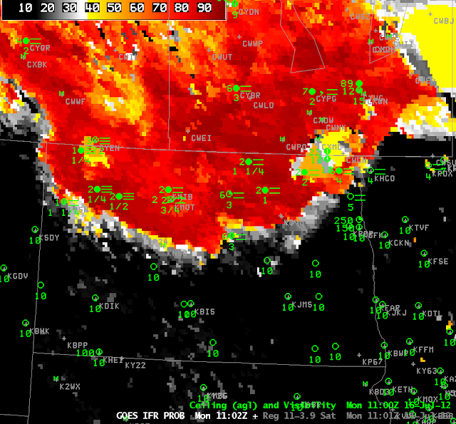
GOES-R IFR probability product at 0745 UTC on 16 July 2012

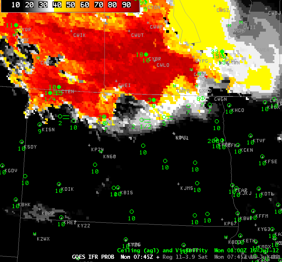
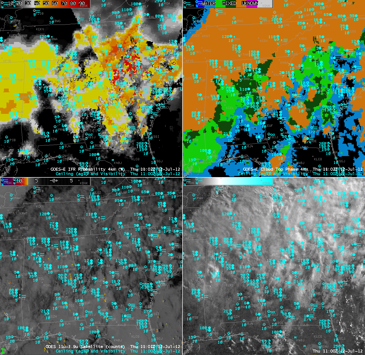
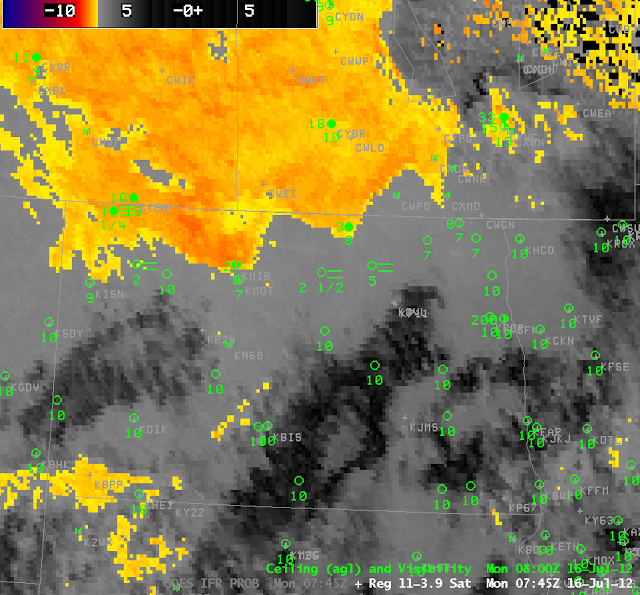
The two images above show the ‘traditional’ GOES fog product — the brightness temperature difference between 11 and 3.9 micrometers — at 0745 UTC on 16 July 2012 (top) and the GOES-R IFR probabilities at the same time.  In addition, ceilings and visibilities at stations in North Dakota are plotted.  Both products accurately capture the fog/low stratus along the North Dakota/Canada border.  The IFR probabilities do a better job at suggesting the development of IFR at Rugby, ND (with 2-1/2 mile visibility).  The IFR probabilities are also correct over southwestern North Dakota: IFR conditions do not exist there despite the brightness temperature difference.

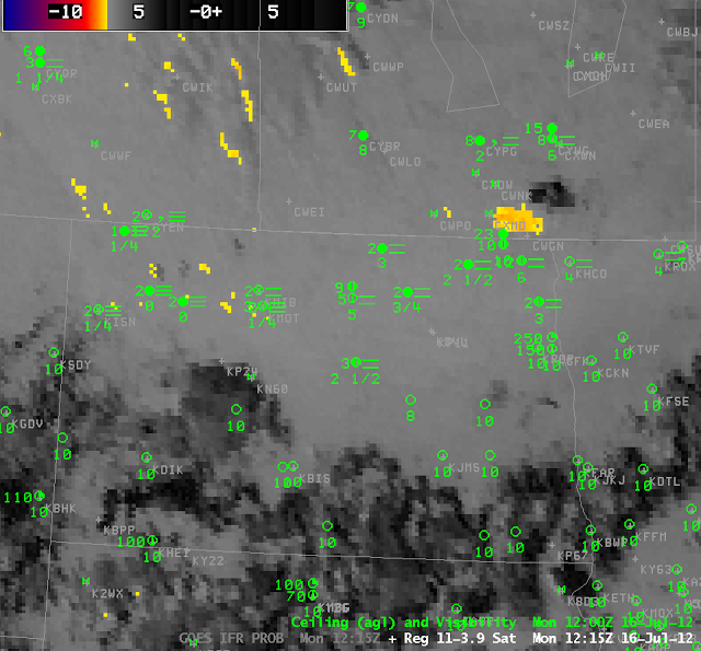
Brightness Temperature Difference (11 micrometers – 3.9 micrometers) at 1101 UTC on 16 July

GOES-R IFR probability product at 1102 UTC on 16 July 2012

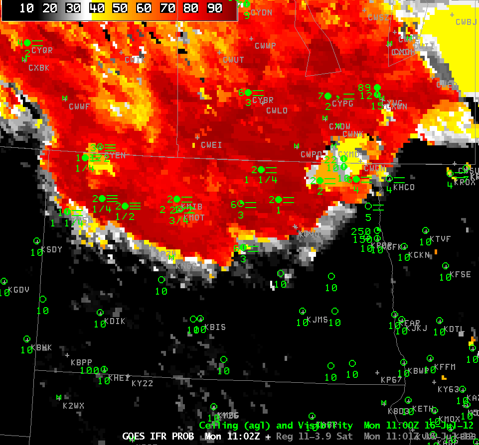
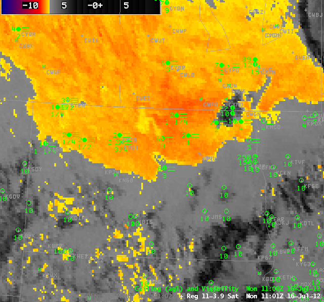
At 1100 UTC (above), both products accurately portray the existence of fog/low stratus over north central North Dakota, but the traditional brightness temperature difference product continues to suggest fog/low stratus over southwestern North Dakota, where IFR conditions do not exist, and where the IFR probability has little signal.

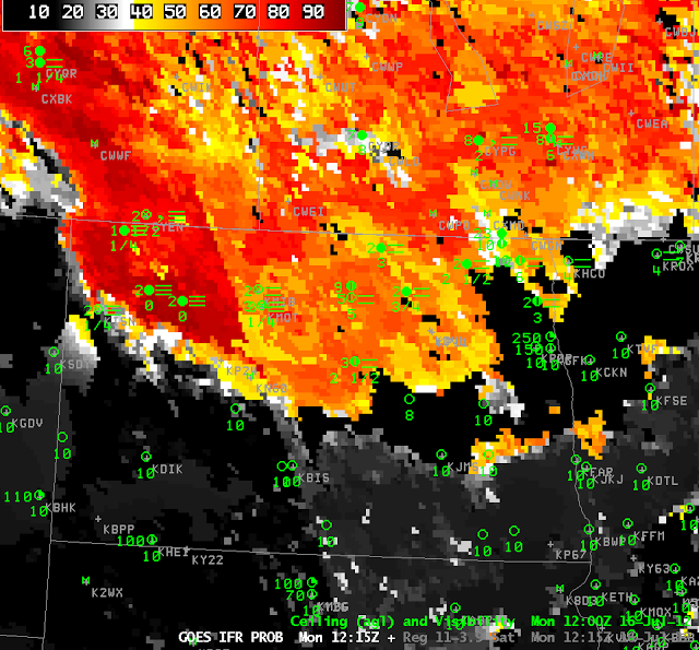
Brightness Temperature Difference (11 micrometers – 3.9 micrometers) at 1215 UTC on 16 July

GOES-R IFR probability product at 1215 UTC on 16 July 2012

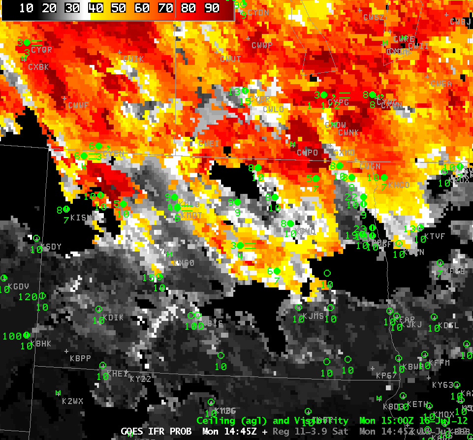
When the sun rises, reflected solar 3.9-micrometer radiation causes the brightness temperature difference between 11 and 3.9 micrometers to flip sign, and the color enhancement used at night loses value in day.  In contrast, the GOES-R IFR probability maintains a robust signal from nighttime through twilight to daytime (the terminator is visible in the IFR probability image at 1215 UTC 16 July, above, running north-northwest from south-central North Dakota to western north-central North Dakota).  Higher IFR probabilities continue to overlap the region where IFR conditions are reported.  By 1445 UTC (below), the region of IFR conditions is breaking apart;  stations that persist in reporting IFR conditions (or near IFR) are within the highest IFR probability in the field — Minot and Harvey in ND, Estevan in Saskatchewan and Portage in Manitoba.

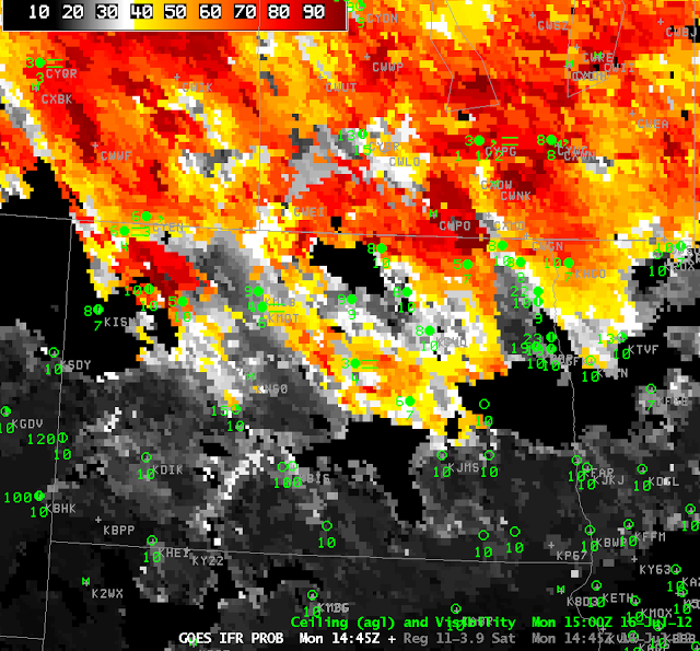
GOES-R IFR probability product at 1445 UTC on 16 July 2012

Fog and Low Stratus where it rains

Fog and low stratus is not rare in regions of precipitation, but the brightness temperature difference algorithm used historically to infer fog will not highlight such areas as those where IFR conditions are likely, usually because the emissivity properties of the precipitating clouds differ from those of fog/stratus decks.  The GOES-R Fog/Low Stratus product nevertheless will produce a signal in these regions because it uses input from numerical models in regions where a satellite signal cannot provide information.
GOES-East IFR Probabilities from the GOES-R Fog/Low Stratus algorithm (upper left), GOES-East cloud phase (upper right), GOES-East brightness temperature difference (11 microns – 3.9 microns) (lower left), GOES-East visible imagery (enhanced for low light conditions) (lower right), all for 1100 UTC on 12 July 2012.

Several things require explanation in these images.  In the IFR probability mapping, the SSE to NNW boundary extending from near Jacksonville to Chattanooga is the terminator, the boundary between using nigthtime and daytime values in the look-up tables that are used to relate model and satellite fields to IFR probabilities.  Note that the daytime values generally yield higher probabilities than the nighttime values, especially for regions where IFR probabilities are determined mostly from model output.  Regions where that occurs — where model output drives the IFR probability output — are typically underneath widespread ice clouds, and the probability fields have a more uniform look to them.  In the image above, more satellite data are being used over South Carolina, and the resultant IFR probability field has a more pixelated character.  Note, however, how little information about fog and low stratus is present in the traditional brightness temperature difference field in the lower left.  IFR flight rules are common from south central Georgia northeastward into South Carolina and over northern Mississippi.