Category Archives: Southeast

IFR Probability Motion as a forecast tool

ifrprobability_13oct2016_0200_1407anim

GOES-R IFR Probability Fields, 0200-1400 UTC on 13 October 2016 along with surface observations of ceilings/visibility (Click to enlarge)

Because GOES-R IFR Probability fields are computed with the same time latency as GOES imagery, motion of the IFR Probability fields can have predictive value.  In the animation above, higher GOES-R IFR Probability  is moving eastward;  IFR Conditions are reported as the higher IFR conditions move overhead (consider, for example, Bowling Green, KY, or Clarksville, TN), and ceilings / visibilities improve as the band of higher IFR conditions moves eastward from a station (over southern Illinois, for example).

Fog after convection in Virginia and North Carolina

ifrp_28sept2016_0215_1125anim

GOES-R IFR Probability fields, hourly from 0215 UTC through 1115 UTC on 28 September 2016 (Click to enlarge)

IFR and Low IFR Conditions developed over parts of Virginia and the Carolinas Piedmont Region during the morning of 28 September 2016. The screengrab below, from the Aviation Weather Center, shows the areal extent of the reduced visibilities and/or low ceilings.  (The text of the IFR Sigmet is here.)  Fog over southeastern  Virginia is developing under multiple cloud decks associated with the convection near a front.  IFR Probabiities in this region are determined by Rapid Refresh data that shows low-level saturation; the flat-looking field over that region is characteristic of model-only IFR Probability fields.  Farther to the southwest, over western North Carolina, IFR Probabilities are determined by both satellite and model data;  notice how pixelated the data are in that region.

awc_1213utc_28sept

Screengrab from the Aviation Weather Center at 1215 UTC on 28 September 2016 (Click to enlarge)

Suomi NPP overflew the eastern United States shortly after 0730 UTC, and the toggle below shows the Day Night Visible Band and the Brightness Temperature Difference field (11.45 – 3.74 ).   Water-based clouds (yellow and orange in the enhancement used) are detected just to the west of cirrus and mixed-phase clouds (black in the enhancement used).  The 0737 UTC IFR Probability field, at bottom, had model-data only as predictors in regions where Suomi NPP shows multiple cloud layers.  Note also that the 1-km resolution of Suomi NPP is resolving the developing valley fogs in the Appalachian mountains of Ohio, West Virginia and Kentucky.  There are only a few pixels in the IFR Probability field that are suggesting valley fog development — but note in the end of the animation at the top of this post that more valley pixels show IFR Probability signals.  When GOES-R is flying, its superior (to GOES-13) 2-km resolution should mitigate this too-slow identification of valley fogs.

snpp_btd_dnb_0736_28sep2016toggle

Suomi NPP Day Night Band Visible (0.70) and Brightness Temperature Difference (11.45 – 3.74) fields at 0736 UTC on 28 September 2016 (Click to enlarge)

ifrp_28sept2016-35

GOES-R IFR Probability fields at 0737 UTC, and surface observations of ceilings and visibilities at 0800 UTC (Click to enlarge)

Radiation Fog over South Carolina

goesr_ifrp_13sept2016anim_0200_1000

GOES-R IFR Probability Fields and surface reports of ceilings and visibilities, 0100-1000 UTC on 13 September 2016 (Click to enlarge)

High Pressure over the eastern United States allowed Radiation Fog to form over much of the southeast early on the morning of 13 September 2016.  The GOES-R IFR Probability hourly animation, above, shows increasing probabilities of IFR conditions over much of North and South Carolina, with IFR conditions observed at many stations by sunrise (graphic from here).  IFR Probabilities provided an earlier alert to the fog development (as such, it’s a good situational awareness tool) than was possible from the traditional brightness temperature difference field (see the 0400 UTC image below — click here for a much larger image) because of multiple cloud layers present over the Carolinas in the wake of departing showers. The enhancement for the brightness temperature difference field is such that clouds composed of water droplets are typically shaded orange or yellow.  In the 0400 UTC brightness temperature difference field below (right), fog is not indicated over South Carolina.

tifrp_btd_0400_13sept

GOES-R IFR Probability fields (left) and GOES-13 Brightness Temperature Difference Fields (right), both from 0400 UTC on 13 September 2016 (Click to enlarge)

GOES-R Cloud Thickness fields can be used to estimate fog dissipation time for radiation fog. This scatterplot shows a rough relationship between the last thickness field produced before twilight conditions and the dissipation time. That field is shown below — note that portions of eastern North Carolina have slipped into twilight conditions already by 1100 UTC. Maximum values over South Carolina are around 850 feet (near Greenville/Spartanburg), while those over North Carolina exceed 1200 (near Asheville). Fog dissipation should occur first over South Carolina, then over North Carolina.

goes_r_cloudthickness_1100_13sept

GOES-R Cloud Thickness Field, 1100 UTC on 13 September 2016 (Click to enlarge)

IFR Probability and Aviation

GOES_IFR_P_1400_5August2016

GOES-R IFR Probability, 1400 UTC on 5 August 2016, along with surface reports of ceilings and visibilities (Click to enlarge)

GOES-R IFR Probability describes regions where IFR Conditions are likely. For example, the IFR Probability field above, from 1400 UTC on 5 August 2016, shows high probabilities over part of the Piedmont from Virginia southwestward into Georgia.  Observations confirm that IFR Conditions (and near-IFR conditions) exist in this region of higher probabilities.

The Aviation Weather Center maintains a website with products that dovetail nicely with IFR Probability fields.  For example, the screenshot below shows stations reporting IFR Conditions (in red) and Low IFR Conditions (in magenta) ( a CWA-issued polygon on IFR conditions is included).  The overall extent of the IFR Conditions in the image above and plotted below is also roughly similar.  The G-AIRMET of IFR Conditions, bottom, also shows overlap with the IFR Probability field, as expected.

AviationScreenShot

Aviation Weather Center screenshot from 1456 UTC showing region of IFR and Low IFR Probability over the southeastern and mid-atlantic states (Click to enlarge)

AIRMETAviationScreenShot

Graphical Depiction of IFR G-AIRMET and MTN OBS (Mountaintop Obscuration) G-AIRMET at 1500 UTC on 5 August 2016 (Click to enlarge)

Near-IFR conditions over South Carolina

4Panel_IFR_BTD_CLDTHICK_WV_VIS_0300_1400anim

GOES-R IFR Probability (Upper Left), GOES-R Cloud Thickness (Lower Left), GOES-East Brightness Temperature Difference (10.7µm – 3.9µm) (Upper Right), GOES-East Water Vapor (6.5µm) at night, Visible Imagery (0.65µm) in day (Lower Right), hourly from 0315 UTC through 1400 UTC 29 January 2015 (Click to enlarge)

The animation above shows hourly imagery, from 0315 through 1400 UTC on 29 January 2016 (Click here for a faster animation). GOES-R IFR Probabilities are moving northeastward from South Carolina into North Carolina throughout the animation. Changes in surface observations of ceilings and visibilities closely match the motion of the GOES-R IFR Probability field. This is a case where the GOES-13 Brightness Temperature Field also is giving information about the presence of low clouds; GOES-R IFR Probability lends confidence to a forecaster that the stratus deck is actually fog because GOES-R IFR Probability includes information about low-level saturation (from the Rapid Refresh Model that is one of the predictors used in the statistical model used to generate IFR Probability fields).

In the early part of the animation, higher clouds are present and can be detected both in the water vapor imagery and in the brightness temperature difference (high clouds are dark in the enhancement curve used). When high clouds are present, GOES-R Cloud Thickness (in the lower left of the figures above) will not be determined as it is derived from an empirical relationship between the 3.9 emissivity of low clouds and cloud thickness that was determined from sodar observations of cloud thickness off the West Coast of the USA. High clouds prevent a determination of this relationship. Regions where GOES-R Cloud Thickness is not computed at night because of high clouds correspond very well with regions where GOES-R IFR Probability is determined by Rapid Refresh Model Output only.

IFR Probabilities give information during the day too

IFRPROB_24Sep2015_13-17anim

GOES-R IFR Probabilities, hourly from 1300-1700 UTC on 24 September 2015 (Click to enlarge)

Ceilings and visibilities over South Carolina decreased during the day on 24 September 2015. The animation of hourly IFR Probability fields, above, shows an increase in Probability over South Carolina as the visibilities decreased.  IFR Probability fields can alert a forecaster to the possibility of IFR conditions at any time of the day.   Visible imagery for the same period, below, shows the multiple cloud layers streaming inland. The accuracy of the IFR Probability field in highlighting the region with near-IFR and IFR Probability is testimony to the accuracy of the Rapid Refresh model data that are used.

VIS_1300_1700_24sept2015anim

GOES-East Visible (0.63 µm) Imagery, hourly from 1300-1700 UTC on 24 September 2015 (Click to enlarge)

IFR Probability and fog over the Southeast United States

This blog post shows how IFR Probability fields can give an early alert to the development of IFR Conditions.

SouthEast_24August2015_0400

GOES-R IFR Probability fields, 0400 UTC 24 August 2015 (Click to enlarge)

GOES-R IFR Probability fields from 0400 UTC on 24 August 2015, above, show enhanced probabilities over interior southeast Georgia.  Observations of surface visibilities and ceilings do not show widespread IFR conditions.   But the presence of enhanced values in IFR Probability suggest careful attention should be paid to this region.

SouthEast_24August2015_0700

GOES-R IFR Probability fields, 0700 UTC 24 August 2015 (Click to enlarge)

Three hours later (0700 UTC), IFR Probabilities have increased somewhat, and some observations are closer to IFR conditions.  This is consistent with the slow development of radiation fog overnight over the southeast part of the country.

SouthEast_24August2015_0915

GOES-R IFR Probability fields, 0915 UTC 24 August 2015 (Click to enlarge)

By 0915 UTC, above, IFR Conditions are observed in regions where IFR Probabilities continue to increase. The increase in IFR Probability values continues at 1100 UTC, below, with numerous regions with values exceeding 90%. IFR Conditions are widespread over southeast Georgia and parts of adjacent South Carolina.

SouthEast_24August2015_1100

GOES-R IFR Probability fields, 1100 UTC on 24 August 2015 (Click to enlarge)

SouthEast_24August2015_1300

IFR Probability fields are consistent through sunrise, with values exceeding 90% after the sun has risen, at 1300 UTC, above. The cloud-clearing that can be done with visible imagery at 1300 UTC means the edges of the fog field are more sharply defined at 1300 UTC than they were at 1100 UTC.

Dense Fog in South Carolina and Georgia

DenseFog_4Aug2015

Screenshot from Charleston WFO, 1230 UTC 4 August 2015

GOES_R_IFRP_0400_1215_4Aug2015anim

GOES-R IFR Probability fields computed from GOES-13 and Rapid Refresh Data, hourly from 0400 through 1215 UTC 4 August 2015 (Click to enlarge)

Dense fog developed over the piedmont of South Carolina/Georgia on 4 August 2015 in the wake of departing convection. The GOES-R IFR Probability fields, shown above hourly from 0400 to 1215, do parallel the development of the reduced ceilings and visibilities. Brightness Temperature Difference fields, below, from 0615 to 1215 UTC, do not show a strong fog signal until after 0800 UTC, yet IFR conditions at that time stretch from Walterboro SC (KRBW) southeastward to Eastman GA (KEZM) and Baxley GA (KBHC). GOES-R IFR Probabilities therefore give a better head’s up to a forecaster tasked with monitoring ceilings and visibilities.

GOES_BTD_0615_1215_4Aug2015anim

Suomi NPP overflew the Southeast United States at ~0730 UTC on 4 August. Ample illumination from the waning three-quarter moon showed cloudiness over southeastern coastal South Carolina and adjacent parts of Georgia but the brightness temperature difference field does not suggest that these are all water-based clouds (such clouds generally fall in the yellow or orange part of the enhancement).

SNPP_DNB_0732_04Aug2015

Suomi NPP Day Night Band visible (0.70 µm) image, 0732 UTC 04 August 2015 (click to enlarge)

SNPP_BTD_0732_04Aug2015

Suomi NPP Brightness temperature Difference field (11.45 µm – 3.74 µm), 0732 UTC on 4 August 2015 (click to enlarge)

MODIS data from Terra and Aqua satellites can also be used to compute GOES-R IFR Probability fields, and two MODIS swaths were produced over South Carolina/Georgia early on August 4. Toggles between the 0337 Terra-based GOES-R IFR Probability Field and the 0755 UTC Aqua-based GOES-R IFR Probability fields are below. The larger values from MODIS — especially at 0755 UTC — suggest the fog was initially at small-scale horizontally. The 1-km resolution pixels from MODIS better capture any small-scale features.

GOESMODIS_IFRP_0337_4Aug2015toggle

MODIS-based (Terra) and GOES-based (GOES-13) GOES-R IFR Probability fields at ~0340 UTC on 04 August 2015 (click to enlarge)

GOESMODIS_IFRP_0755_4Aug2015toggle

MODIS-based (Aqua) and GOES-based (GOES-13) GOES-R IFR Probability fields at ~0800 UTC on 04 August 2015 (click to enlarge)

IFR Conditions over the Southeast United States

US_11-3.9_Sat_20150302anim

Brightness Temperature Difference Fields (10.7µm – 3.9µm) from GOES-East, hourly from 0400-1300 UTC on 2 March 2015 (Click to enlarge)

A series of frontal systems along the east coast caused multiple cloud layers and IFR conditions over much of the deep south and piedmont from Mississippi to Georgia and up through Virginia overnight on 1-2 March 2015. The animation of Brightness Temperature Difference (10.7µm – 3.9µm), above, is testimony to the difficulty in using that product as a fog detection device when multiple cloud layers are present: Many stations underneath cirrus show IFR Conditions. (Note also how the signal changes at 1300 UTC — the end of the animation — as the sun rises and increasing amounts of 3.9µm solar radiation is reflected off the clouds).

The GOES-R IFR Probability fields, below, better identify regions of reduced visibility underneath mixed cloud layers. It does this by incorporating model data (from the Rapid Refresh) into its suite of predictors. Thus, where low-level saturation is indicated under multiple cloud layers, IFR Conditions can be assumed to be occurring, and computed IFR Probabilities are large. The hourly animation of GOES-R IFR Probability, below, shows a good overlap between large IFR Probabilities and IFR (or near-IFR conditions). The flat IFR Probability field that is widespread over the Piedmont region of the Carolinas is typical of an IFR Probability field determined mostly by model output. Where high clouds break, pixelated regions develop (and IFR Probabilities increase) in the field.

GOES_IFR_PROB_20150302anim

GOES-R IFR Probability fields, 0400-1300 UTC on 2 March (Click to enlarge)

The 1215 UTC and 1300 UTC imagery in the IFR Probability animation above include a discernible nearly north-south line. (The 1215 UTC image is below).  This is the terminator.  To the right of that line, where IFR Probabilities are slightly larger (dark orange), daytime predictors are being used;  to the left of that line, IFR Probabilities are slightly smaller (lighter orange) and nighttime predictors are being used.  Why is the probability a bit larger in the daytime predictors?  In part this is because visible imagery can be used to ascertain whether clouds are present.  You can be a bit more confident that IFR conditions are present because clouds are present in the visible imagery.

GOES_IFR_PROB_20150302_1215

GOES-R IFR Probability fields, 1215 UTC on 2 March (Click to enlarge)


Traffic-snarling fog in Huntsville, Alabama

AlabamaFog

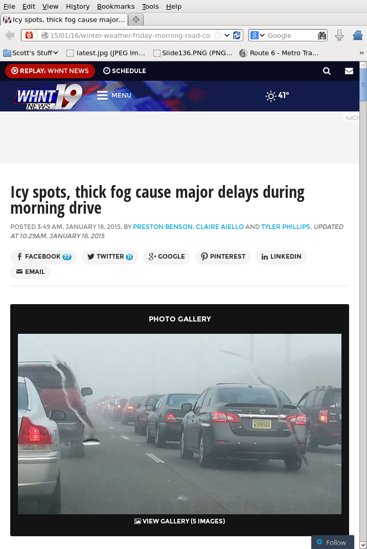
Dense fog developed over the Tennessee River Valley during the morning hours of 16 January 2015, causing crashes and traffic and school delays. The screenshot above (from this link), from WHNT in Huntsville, shows the conditions.

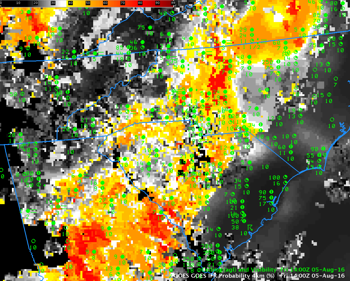
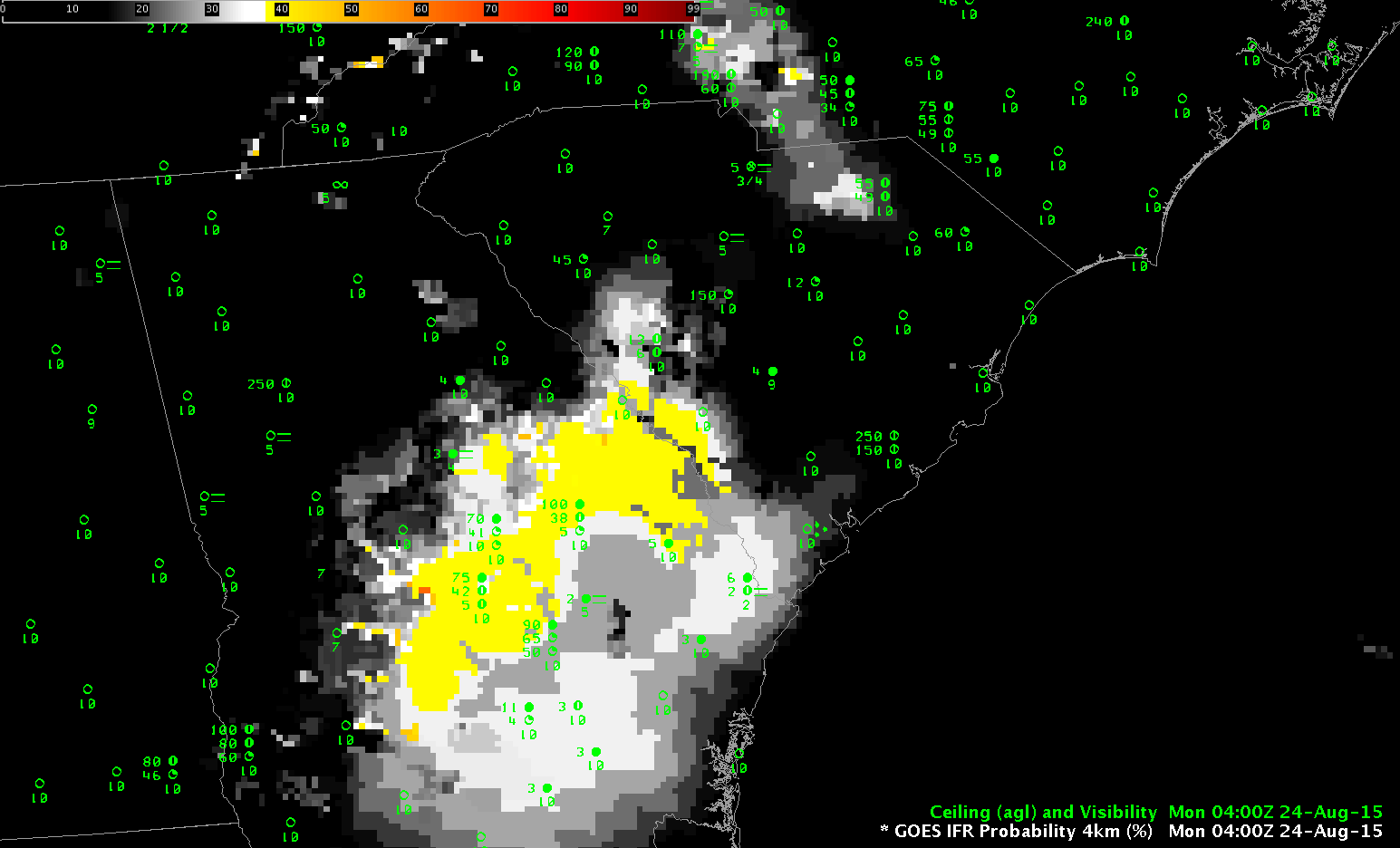
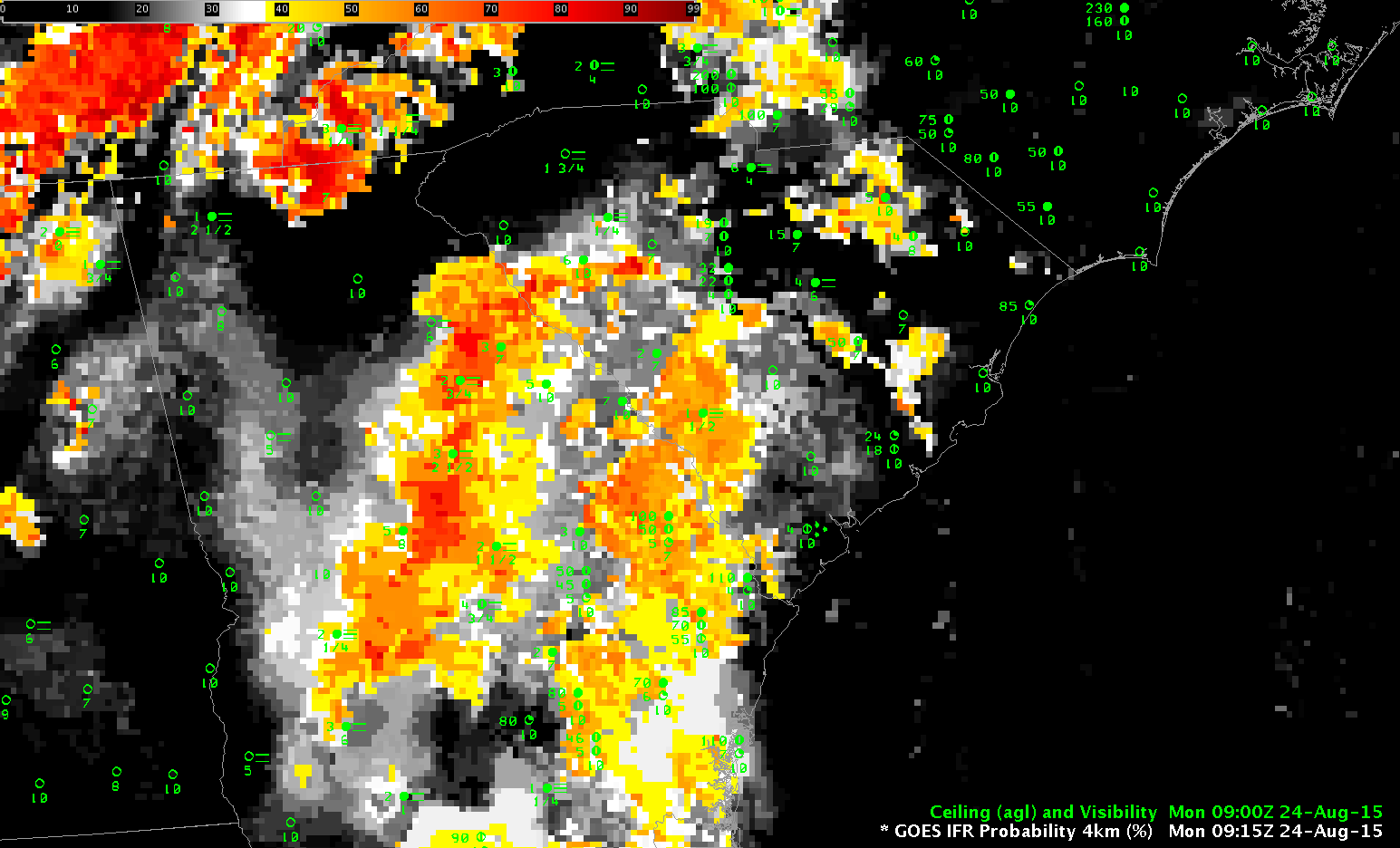
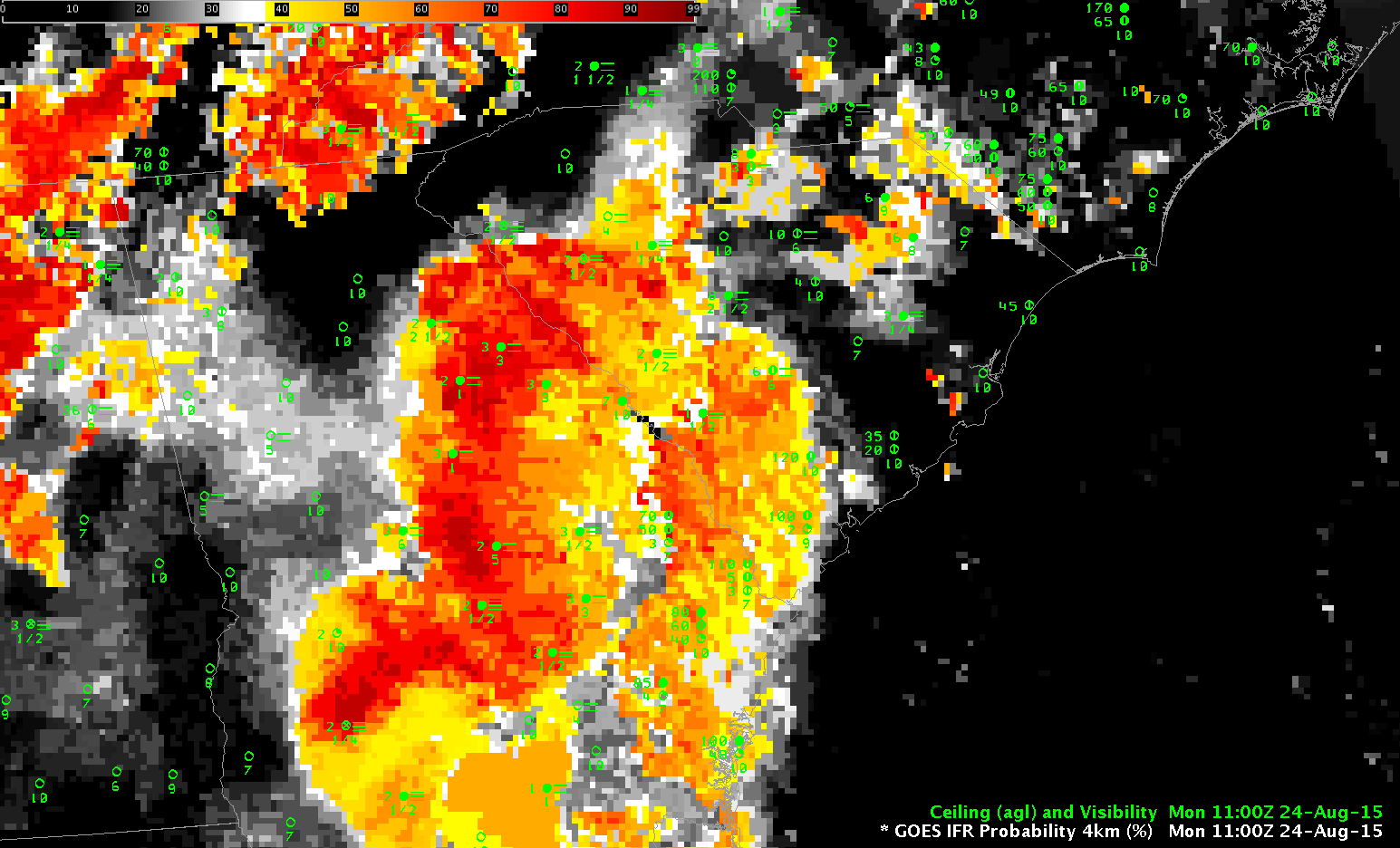
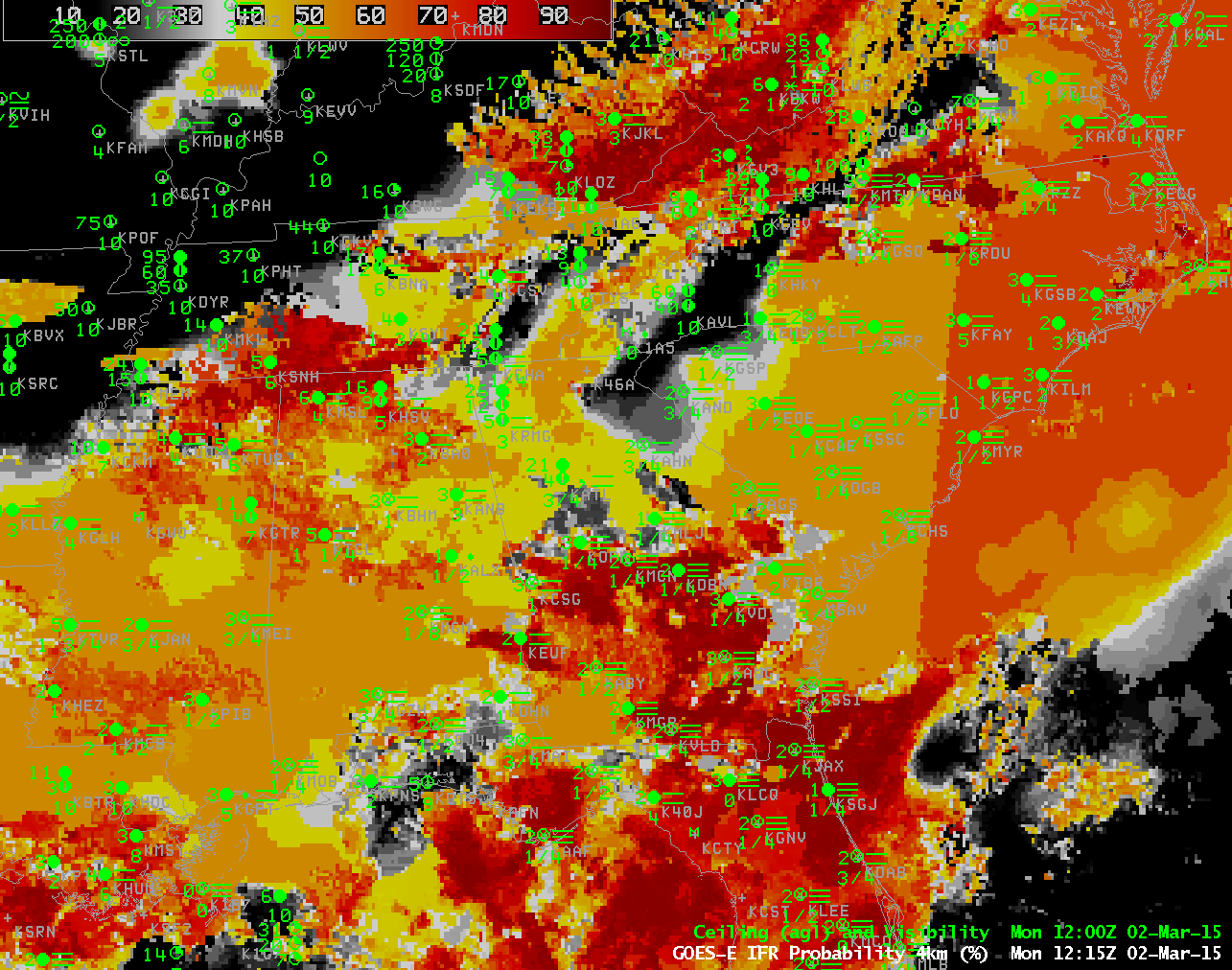
IFR Probability Fields, below, show a large stratus deck moving southward over Alabama, moving south of Hunstville by 0700 UTC. Clear skies allowed additional cooling and a radiation fog developed. The fog impeded transportation in and around Huntsville. IFR Probabilities increased around Huntsville after the large-scale stratus deck moved out, and remained high until around 1500 UTC when all fog dissipated. IFR Probability fields are computed using both satellite data and Rapid Refresh Model data. That IFR Probability is high over Huntsville and surroundings as the fog develops says that satellite data suggests water cloud development and that model data suggests near-surface saturation.

GOES_IFR_PROB_20150116

GOES-R IFR Probabilities, half-hourly imagery, 0415-1645 UTC, 16 January 2015 (Click to enlarge)

The fog was also diagnosed using traditional detection methods, such as the brightness temperature difference field from GOES-13 shown below. Brightness Temperature Difference fields detect both fog and elevated stratus, and it’s difficult for satellite data-only products to distinguish between the two cloud types because no surface information is included in a simple brightness temperature difference field.

US_11-3.9_Sat_20150116

GOES-13 Brightness Temperature Differences (10.7µm – 3.9µm), half-hourly imagery, 0410-1645 UTC, 16 January 2015 (Click to enlarge)

For a small-scale event such as this, polar orbiting satellites can give sufficient horizontal resolution to give important information. MODIS data from Terra or Aqua can be used to compute IFR Probabilities, and a toggle between the MODIS brightness temperature difference field, and the MODIS-based IFR Probabilities at 0704 UTC is below; unfortunately, Terra and Aqua were not overhead when the fog was at its most dense, but a thin filament of fog/High IFR Probability is developing south of Huntsville in a river valley.

MODIS_IFR_PROB_BTD_20150116_0704

MODIS Brightness Temperature Difference and MODIS-based IFR Probabilities at 0704 UTC on 16 January 2015 (Click to enlarge)

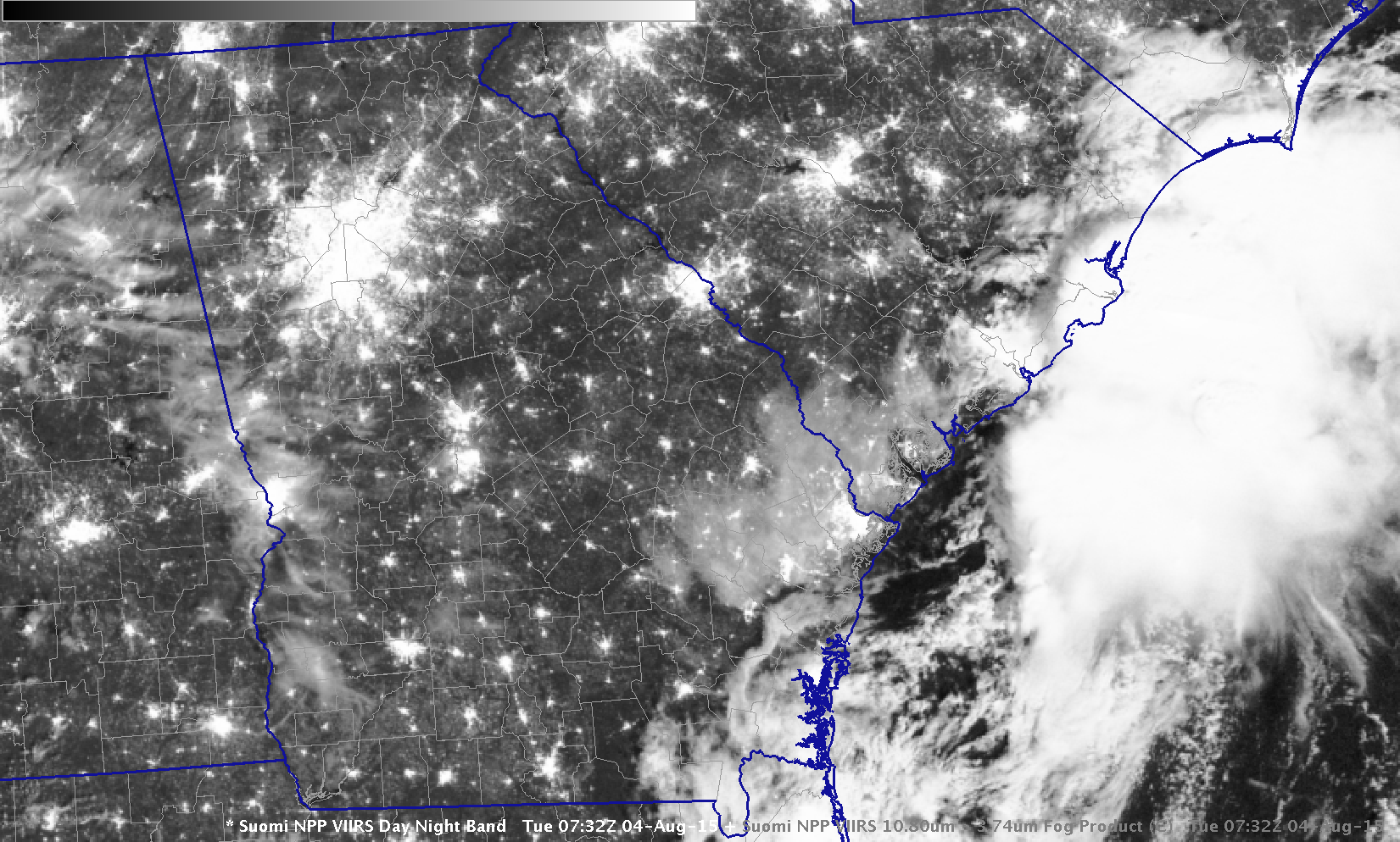
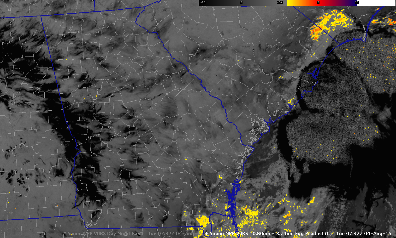
Suomi NPP was positioned such that northern Alabama was viewed on two successive orbits, and the toggle below shows the brightness temperature difference field (11.35 – 3.74). Similar to GOES, Suomi NPP Brightness Temperature Difference fields show the development of water-based clouds in/around Huntsville.

VIIRS_FOG_20150116_0645_0828

Suomi NPP Brightness Temperature Difference fields at 0645 and 0828 UTC, 16 January 2015 (Click to enlarge)