GOES-17 IFR Probability around Bristol and Kvichak Bays

GOES-17 IFR Probability, 0820 – 1800 UTC on 17 November 2020 (Click to enlarge)

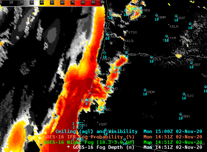
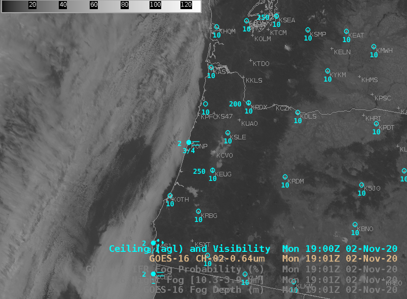
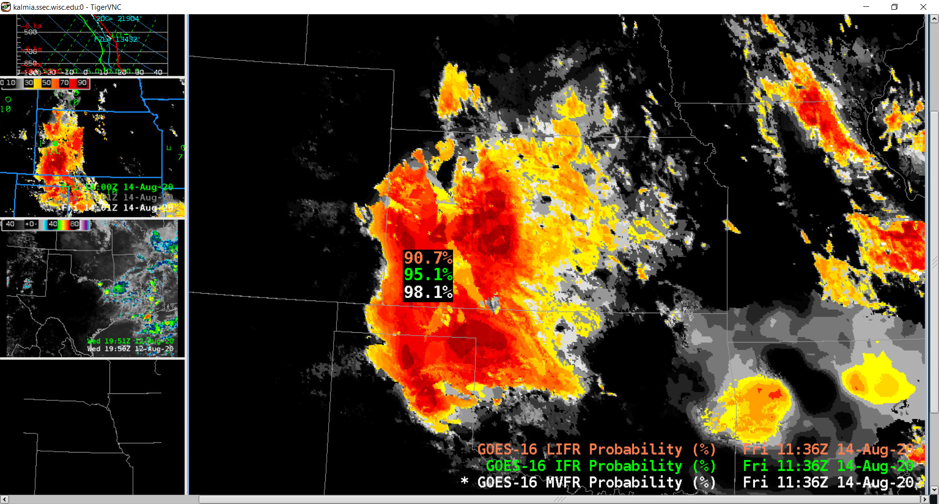
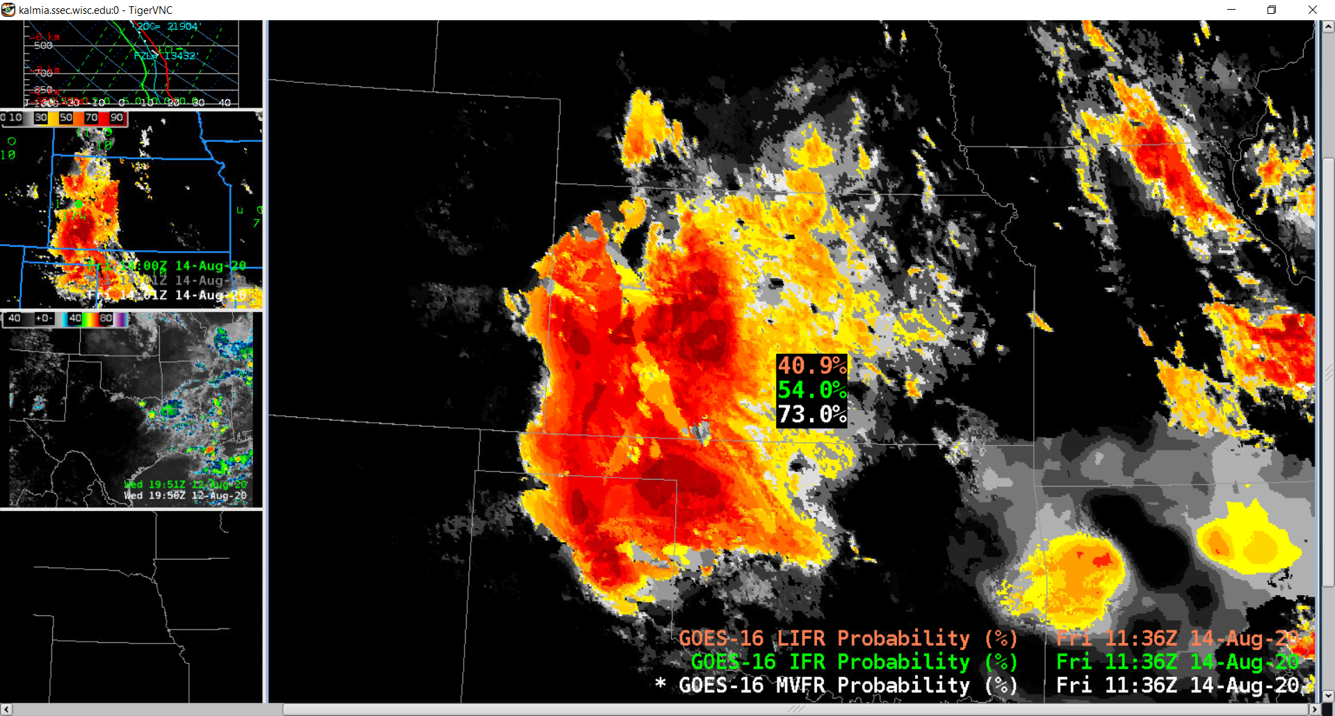
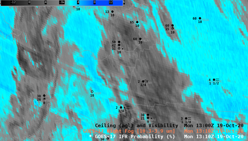
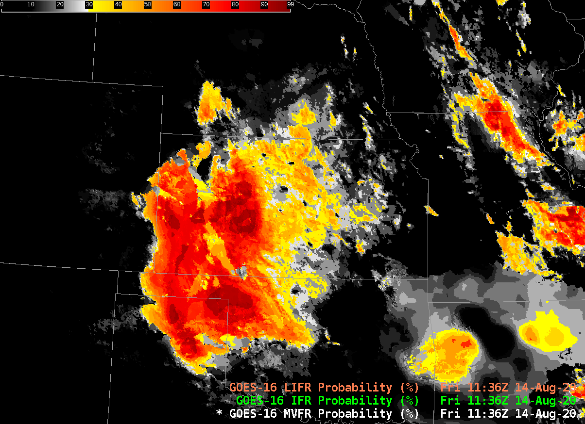
GOES-17 IFR Probability fields, above, show a thin region along the northern shore of Bristol and Kvichak Bays in southwestern Alaska, north of the Aleutian Peninsula, where IFR conditions are likely . Probabilities are highest around King Salmon (PAKN) and Igiugig (PAIG) northeast of King Salmon. Several nearby airports are not reporting observations (PAII — Egegik — just south of King Salmon; PATG –Togiak — along the northern shore of the Bay, east of PAEH (Cape Newenham). IFR probability uses satellite and model information to create an estimate of whether or not IFR conditions will be met in regions where observations are missing. Sometimes, as over Cape Newenham at the end of the animation, high clouds are present and only model data can be used to create the estimate.

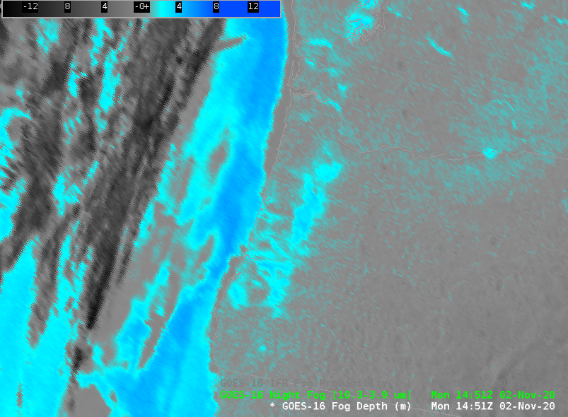
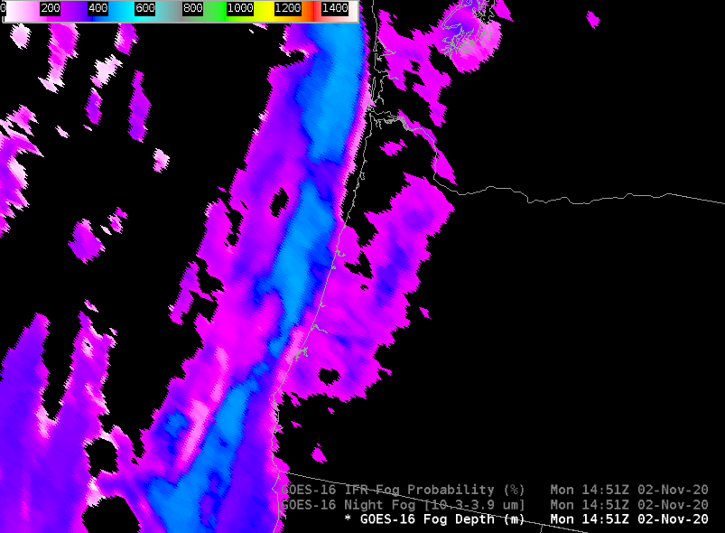
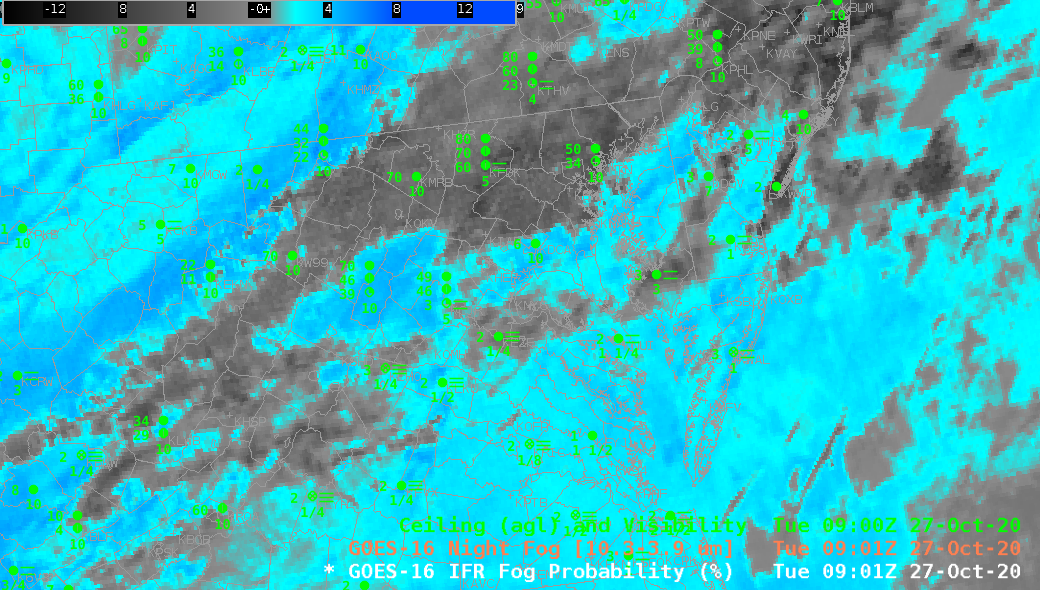
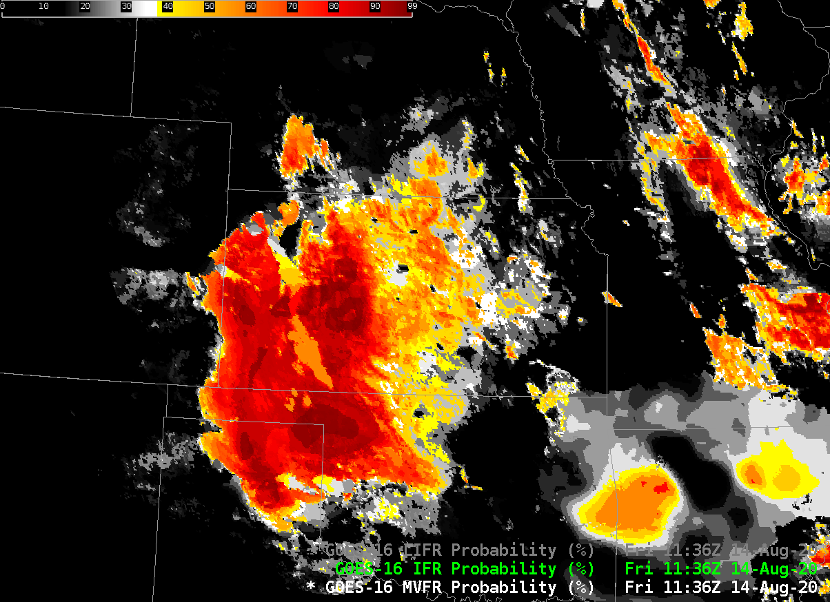
The Night Fog Brightness Temperature Difference field, below, shows that low clouds (made up of water droplets) exist over the same region — but this one product cannot indicate whether the stratus deck observed is reducing visibility near the surface (where aviation interests require that information). The model data that are incorporated into IFR Probability in concert with satellite data allow for a better estimate of where visibility is reduced than do satellite data alone. This is especially important when the presence of high clouds, as at the end of the animation in the western part of this domain, makes it difficult for the satellite to view low clouds.

GOES-17 ‘Night Fog’ Brightness Temperature Difference field (10.3 µm – 3.9 µm), 0820-1800 UTC on 17 November 2020 (Click to enlarge)
IFR Probability, Low IFR Probability, and Night Fog Brightness Temperature difference at 1000 UTC on 17 November 2020 (Click to enlarge)

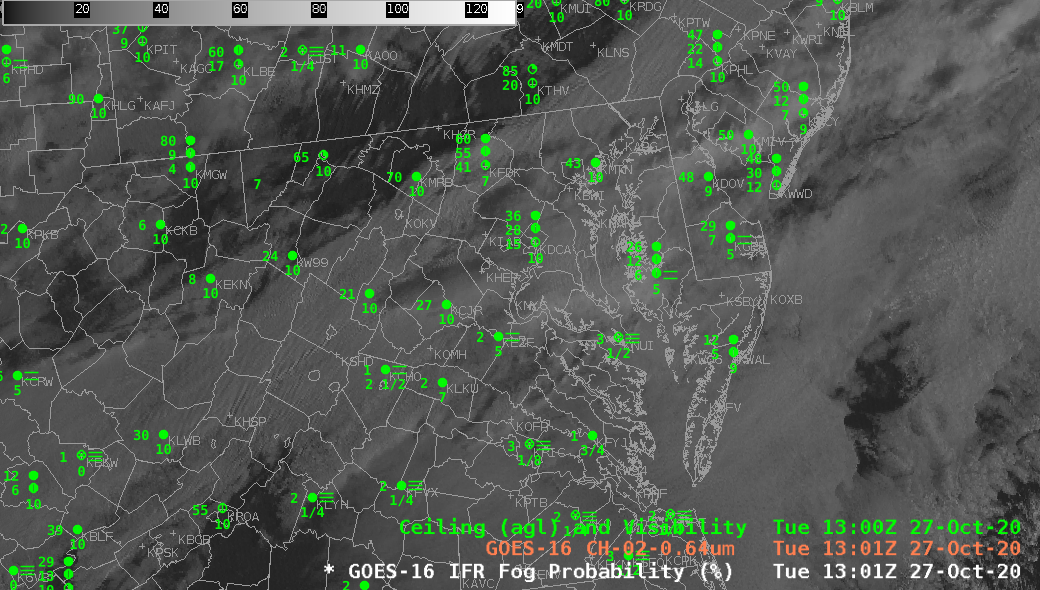
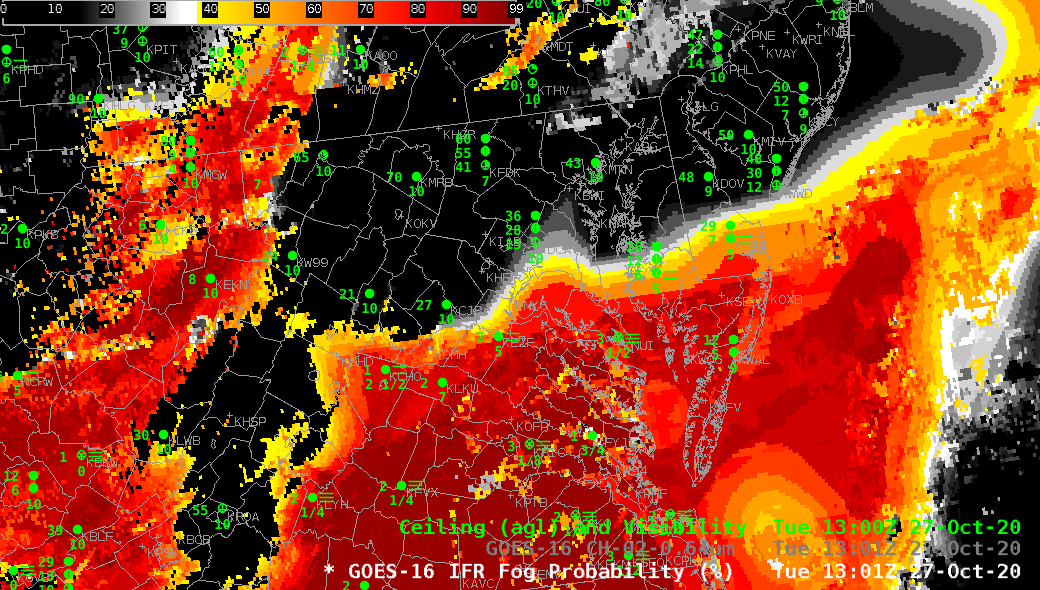
Toggles at 1000 UTC (above) and 1600 UTC (below) of IFR Probability, Low IFR Probability and Night Fog Brightness Temperature Difference, suggest that the greatest likehihood of reduced visibilities are not along the bay shore, but rather inland along the Kvichak River.

IFR Probability, Low IFR Probability, and Night Fog Brightness Temperature difference at 1600 UTC on 17 November 2020 (Click to enlarge)

Fog in Oregon’s Willamette Valley

GOES-16 IFR Probability, 1451 UTC on 2 November 2020 along with 1500 UTC observations of ceilings and surface visibility (Click to enlarge)

GOES-16 IFR Probability fields, above, show very high IFR Probability values over the Willamette Valley of Oregon to the south of Portland; surface observations in the region show IFR conditions from Salem (KSLE) southward through Eugene (KEUG) to Roseburg (KRBG). IFR Probability is also large along the coast, with IFR conditions reported at Newport (KONP) and North Bend (KOTH). The 10.3 µm – 3.9 µm “Night Fog” Brightness Temperature Difference field, below, also has a modest signal in the Valley, and along the coast, giving a qualitative (but not quantitative) estimate of fog.

GOES-16 Night Fog Brightness Temperature Difference (10.3 µm – 3.9 µm) at 1451 UTC on 2 November 2020 (Click to enlarge)
GOES-16 Cloud Thickness (“Fog Depth”) from 1451-1506 UTC on 2 November 2020 (Click to enlarge)

GOES-R Cloud Thickness (labeled as Fog Depth in TOWR-S Build 19) can be used to estimate radiation fog dissipation time. Values are not computed during the time of rapidly-changing reflected solar radiance (i.e., for the times around sunrise and sunset); the last pre-sunrise value can be used in concert with this scatterplot to estimate burn-off times. Values at 1451 UTC in the Willamette valley peak at around 380 m. This suggests a burn-off time (if this is radiation fog and not advection fog) of about two hours according to the scatterplot below, i.e., shortly before 1700 UTC.

Scatterplot: Last pre-sunrise Cloud Thickness value vs. Dissipation Time. (Click to enlarge)

Visible imagery, below, at 1601 and 1706 UTC do show a trend towards clearing. The scatterplot can underestimate clearing time if (1) the sun angle is lower than at the points used to create the scatterplot or (2) if the fog is not strictly a radiation fog. In either event, however, the values from day to day should give useful information. For example, if today’s last pre-sunrise cloud thickness is greater than yesterday’s, then the burn-off time today should be later than yesterday.

GOES-16 Visible (0.64) Imagery and surface observations of ceilings/visibility at 1601 and 1706 UTC on 2 November 2020 (click to enlarge)
GOES-16 Visible (0.64) Imagery and surface observations of ceilings/visibility at 1901 UTC on 2 November 2020 (click to enlarge)

Fog/low stratus dissipated shortly after the 1901 UTC image shown above.

IFR Conditions over Virginia

GOES-16 Night Fog Brightness Temperature Difference (10.3 µm – 3.9 µm) and IFR Probability at 0901 UTC, along with 0900 UTC plots of surface ceilings and visibility (Click to enlarge)

GOES-16 IFR Probability fields, above, from 0901 UTC on 27 October 2020 (in a toggle with the Night Fog Brightness Temperature Difference), outline two regions of likely IFR conditions over Virginia and surrounding states. Southern Virginia shows restricted conditions, as does the high terrain along the spine of the Appalachians, extending up to Johnstown PA. (Surface observations largely agree with IFR Probability fields: IFR Probability is high where ceilings are low and visibilities are restricted; IFR Probability is low in regions where IFR conditions are not occurring).

Night Fog Brightness Temperature Difference fields (10.3 µm – 3.9 µm), struggle to identify regions of IFR conditions — elevated stratus (over western Virginia and western Maryland, for example) has a similar signal to fog over southeastern Virginia. There are also regions of high clouds above the low stratus over Maryland and Virginia surrounding middle Chesapeake Bay. In such regions, high IFR Probability is being driven by Rapid Refresh model predictions of low-level saturation.


Visible imagery (0.64 µm) toggled with the IFR Probability fields at 1301 UTC, below, show how IFR Probability fields can better discriminate between stratus and fog than visible imagery alone.

GOES-16 Band 2 Visible (0.64 µm) and IFR Probability, 1301 UTC on 27 October 2020 (Click to enlarge)

Use IFR Probability fields to identify regions that have low ceilings and reduced visibilities when Visible imagery (in the day) and Night Fog Brightness Temperature difference (at night). During the day time, this can be achieved by displaying both images at once.

GOES-16 IFR Probability underneath the Visible (0.64 µm) imagery, 1301 UTC, 27 October 2020 (with a transparency alpha of 0.9 applied; click to enlarge)

GOES-17 IFR Probability over western Alaska

GOES-17 IFR Probability fields and GOES-17 Night Fog Brightness Temperature Difference (10.3 µm – 3.9 µm), 1310 UTC on 19 October 2020 (Click to enlarge)

CIMSS is now creating GOES_17 IFR Probability fields for Alaska and will presently be distributing them to the Alaska Region. An example of the utility of the products occurred on 19 October over western Alaska. The toggle above between the Night Fog brightness temperature difference field and the IFR Probability field at 1310 UTC 19 October shows several regions where IFR Probability refines where ceilings and visibilities might restrict aviation — an important piece of information in Alaska.

The default Night Fog Brightness Temperature enhancement is constructed so that stratiform clouds containing water droplets are colored different shades of blue. Higher clouds are various shades of grey.

Consider station PANV — Anvik, AK, near 62.7 N, 160 W. This is a station reporting IFR conditions, and IFR probabilities are near 80%. However, it is also under high clouds; GOES-17 is prevented from viewing low clouds, but the Rapid Refresh model data used in IFR Probability is showing saturation. Model data fills in regions of IFR conditions where high (of mid-level) clouds prevent the satellite from viewing near-surface clouds. Note how IFR Probability is also able to distinguish — correctly — between the IFR conditions at Anvik with the more benign sky conditions to the north at St. Michaels (PAMK), Unalakleet (PAUN) and Shaktoolik (PFSH) along Norton Sound.

In contrast, station PASM — St. Mary’s AK, near 62 N, 163 W — is beneath a strong signal in the Night Fog brightness temperature difference field. However, IFR conditions are not reported, and IFR probabilities are near 40% (and decreasing abruptly to the south). In this region, IFR Probability fields are screening out a region of mid-level stratus.

Station PAMC — McGrath, AK, near 63 N, 155 W — shows near-IFR conditions with a local minimum IFR Probability near 40% and a strong signal of stratus clouds in the Night Fog Brightness Temperature difference. For this station it would be prudent to see how IFR Probabilities were changing with time.

IFR Probability combines the strengths of satellite detection of low clouds with the strength of Rapid Refresh model predictions of low-level saturation to create a product useful in regimes with single or multiple cloud layers.

IFR Probability near a major aviation hub

GOES-16 IFR Probability, 0926 – 1101 UTC on 12 October 2020 (Click to enlarge)

The New York City area has 3 major international hubs for which ceiling/visibility observations and prediction are critical to efficient operations. IFR Probability fields use both satellite data and Rapid Refresh model data and can supply information about low-level conditions even where mid-level or upper-level clouds obscure a satellite’s view of low clouds. The example above shows very slow northeastward progress of an area of potential IFR conditions towards New York.

Satellite-only data, below, in the form of the night fog brightness tempreature difference from GOES-16, does not give a useful signal for the low clouds along the east coast. A conclusion: Use IFR Probability to monitor the progress of low clouds when multiple cloud decks are present.

GOES-16 ‘Night Fog’ Brightness Temperature Difference (10.3 µm – 3.9 µm) field, 1006-1101 UTC, 12 October 2020 with 0900 UTC frontal analysis overlain on first image (Click to enlarge)
GOES-16 IFR Probability and GOES-16 ‘Night Fog’ Brightness Temperature Difference (10.3 µm – 3.9 µm) field, 1101 UTC, 12 October 2020 (Click to enlarge)

The toggle above, between IFR Probability and the Brightness Temperature Difference demonstrates and underscores (1) how IFR Probability can fill in regions under low clouds (in Delmarva and New Jersey, for example), and screen out regions with mid-level stratus (over eastern Lake Ontario the surrounding land, and over eastern Ohio, for example).

IFR Probability fields are supplied to AWIPS (TOWR-S Build 19) via the SBN.

Low Stratus under Cirrus

GOES-16 ‘Night Fog’ Brightness Temperature Difference (10.3 µm – 3.9 µm), 1151 and 1246 UTC on 9 October 2020 (Click to enlarge)

The extensive cirrus shield from Hurricane Delta in the Gulf of Mexico made difficult the satellite-based detection of stratus and low clouds over much of the Deep South on Friday 9 October. The Night Fog Brightness Temperature Difference is also affected by increased solar reflectivity at 1246 UTC in the imagery above. The low clouds over southern Illinois are no longer detected, for example, and the high cirrus of Delta becomes much darker — in both cases because of increased reflectivity of 3.9 µm solar radiation.

The toggle below between the Night Fog Brightness tempreature difference and the Band 4 near-infrared “Cirrus” channel just after sunrise (1246 UTC) shows the extensive cirrus signal in both images. Widespread cirrus is not uncommon, thus the difficulty in detection is not uncommon

GOES-16 Night Fog Brightness Temperature Difference (10.3 µm – 3.9 µm) and near-infrared 1.38 µm “Cirrus” Band 4, 1246 UTC on 9 OCtober 2020 (Click to enlarge)

GOES-R IFR Probability fields, below, compared to the Night Fog Brightness Temperature fields highlight how IFR Probability, which fields include information about low-level saturation in the Rapid Refresh model, capably fills in regions of fog/low stratus underneath high clouds. It is useful for situational awareness in fog detection when satellite imagery is showing only upper-level clouds. For example, note the large values of IFR Probability in western Kentucky, under the high cirrus, or in northeast Texas! There is good spatial correlation between high IFR Probabilities and reduced ceilings/visibilities. The correlation between the Night Fog Brightness Temperature difference field and reduced ceilings/visibilities is smaller because of low visibility under cirrus (as occurring over northwestern TN and much of LA, for example). Note that IFR Probability fields also give information where IFR conditions are not occurring under cirrus: central Mississippi, for example.

GOES-16 IFR Probability and Night Fog Brightness Temperature Difference (10.3 µm – 3.9 µm) at 1151 UTC on 9 October 2020 (Click to enlarge)

IFR Probability fields through sunrise (below) show a consistent signal, in part because of the Rapid Refresh model information on saturation.

GOES-16 IFR Probability fields, 1151 and 1246 UTC on 9 October 2020 (Click to enlarge)

The CIMSS-driven LDM feed that has supplied GOES-16 IFR Probability fields (and before GOES-R’s launch, GOES-13 and GOES-15 IFR Probability fields) to NWS offices will be terminated on or about 20 October. Operational creation of GOES-16 IFR Probability fields has shifted to NOAA/NESDIS, and the fields are now sent over the SBN to forecast offices. TOWR-S Build 19 is required to access and display these fields in AWIPS.

IFR Conditions over the southern Plains

Click to enlarge
GOES-16 Night Fog Brightness Temperature Difference (10.3 µm – 3.9 µm), Night TIme Microphysics RGB, and IFR Probability, 1001 UTC on 22 September 2020 (Click to enlarge)

Widespread mid- and upper-level cloudiness over the southern Plains associated with Tropical Storm Beta on 22 September 2020 make it difficult to use satellite data alone to identify where low clouds and fog might exist. This is a day where IFR conditions exist, as shown here, an image from this website. Where would you expect IFR conditions to exist within this field of view? The Night Fog brightness temperature difference, below, (and, by extension, the Nightime Microphysics RGB) shows scant information over eastern Texas/Oklahoma or ArkLaTex. IFR Probability fields, in contrast, have a definite signal of high probability.

The animation of the Night Fog Brightness Temperature Difference field, below, also highlights a challenge in using this product: increasing reflection of solar 3.9 radiation occurs as sunrise progresses, changing the character of the field. Further, soils can have emissivity properties that are similar to clouds, and a positive Night Fog Brightness Temperature difference signal results. (This is especially true in dry regions, such as west Texas; linked-to map from this website).

GOES-16 Night Fog Brightness Temperature Difference (10.3 µm – 3.9 µm), 0901 – 1306 UTC on 22 September 2020 (Click to enlarge)
GOES-16 IFR Probability, 0901-1306 UTC on 22 September 2020 (Click to enlarge)

IFR Probability fields for the same time as the Night Fog Brightness Temperature Difference, above, show a consistent region where IFR conditions are most likely. The region over the high Plains of Texas that has a signal in the Brightness Temperature Difference field has low probabilities because in that region, the Rapid Refresh model is not suggesting widespread low-level saturation. In contrast, the Rapid Refresh model over east Texas/Oklahoma, western Louisiana and southwest Arkansas does show saturation.

What do observations shows? The hourly observations overlain on the IFR Probability fields, below, show that IFR and near-IFR conditions are widespread within the region of high IFR Probability. Outside that region, IFR conditions are rare.

GOES-R IFR Probability fields, 0906, 1001, 1101, 1201 and 1301 UTC along with observations of ceilings and visibilities (Click to enlarge)

IFR Probability fields are flowing over the SBN to forecast offices. (TOWR-S RPM 19 is needed to display them from that data source). IFR Probability fields are also available via an LDM feed from Regionals if RPM 19 is not installed. They are available online at this website.

GOES-R Fog/Low Stratus Products are now flowing over the SBN

GOES-16 Visible Imagery, 1706 UTC on 9 September, with IFR Probability shown at the same time (with different alpha levels) (Click to enlarge)

GOES-R Fog/Low Stratus Products have been available in NWS Forecast Offices since 2012 via an LDM feed. GOES-16 versions for these products over the CONUS domain are now flowing over the Satellite Broadcast Network (SBN), effective 9 September 2020 (Announcement). Responsibility for this data feed is now at NESDIS following an extensive research-to-operations path. Fields distributed include Probability of: Marginal Visual Flight Rules (MVFR), Instrument Flight Rules (IFR) and Low Instrument Flight Rules (LIFR). In addition to these three probabilities (Click here to see an explanation), there is also a Low Cloud Thickness product that can be used to predict the dissipation time of radiation fogs.

IFR Probabilities, as shown above, are useful because they highlight regions under clouds where visibility restrictions are most likely. Loading it under a visible image and making the visible semi-transparent, as shown above, is a handy way to use the product. A forecaster responsible for transportation concerns can therefore focus their attention where it is needed, as defined by the IFR Probability field: IFR Probability is a good situational awareness tool.

Accessing the Fog/Low Stratus products via the SBN requires TOWR-S RPM v. 19 (It will be baselined in AWIPS v. 21.3.1 in 2021). GOES-17 (and GOES-16) IFR Probabilities are available at this website for the GOES-16 CONUS and GOES-17 PACUS sectors. Work is ongoing to product GOES-17 IFR Probabilities for Alaska.

Fog over western Kansas

GOES-16 Low-IFR Probability, 0846 to 1341 UTC on 14 August 2020 (Click to enlarge)

Fog developed over western Kansas during the early morning of 14 August 2020 (helped along by above-normal precipitation in the past 30 days — shown here in an image created at this website).  Low IFR Probability fields, above, show greatest probabilities of low ceilings and visibility restrictions in regions where they were observed:  over western Kansas, with a sharp cut-off at the Colorado/Kansas border, and over western Oklahoma and the north Texas panhandle.

Compare the evolution of the Low IFR Probability field, above, to the evolution of the Night Fog brightness temperature difference (10.3 µm – 3.9 µm) field below.

  1. The Night Fog field, below, has a region of strong return over western Kansas, but also two regions of weaker signals over central Kansas (where low clouds/fog are observed;  note the regions in the brightness temperature difference field where the signal is very small, small grey pockets within the cyan, corresponding to the locations of towns in central Kansas) and over eastern Colorado (where low clouds/fog are not observed).  Low IFR Probability fields are able to distinguish between the central Kansas and eastern Colorado because model predictions of low-level saturation are used to modulate the satellite-based signal:  Low IFR Probability values are very small over Colorado (where the Rapid Refresh model is not predicting low-level saturation); values are larger over Kansas where ceiling and visibility reductions are occurring and where the Rapid Refresh model is suggesting low-level saturation is present).  The brightness temperature difference field in Colorado might be driven by dry soils rather than low clouds.  A brightness temperature difference signal can emerge at night because of soil emissivity differences (as noted earlier in this blog here).
  2. Low IFR Probability fields are augmented underneath the convection that is apparent in the brightness temperature difference field over northwestern Arkansas.  Satellite detection through the deep convection of low stratus in this region is impossible; the signal is driven by low-level saturation predicted by the Rapid Refresh model output.
  3. As the sun rises, the brightness temperature difference field loses obvious cloud-detection signal because increasing amounts of reflected solar radiation (at 3.9 µm) overwhelm the emissivity-driven difference over low clouds at 3.9 µm and 10.3 µm.  At some point after sunrise, the brightness temperature difference flips sign (and appears dark in the enhancement) because there is far more reflected solar radiation at 3.9 µm than at 10.3 µm.
  4. The Low IFR Probability field by design includes temporal continuity around sunrise and sunset.  This is most noticeable over central Kansas.  The terminator sweep is noticeable in the field, but the values change only slowly in the hour surrounding the terminator.  This temporal continuity is necessary because of the quick changes in detected 3.9 µm radiation that are occurring as solar reflectance changes occur.
GOES-16 Night Fog Brightness Temperature Difference (10.3 µm – 3.9 µm). 0846 to 1341 UTC on 14 August 2020 (Click to enlarge)

The relationship between MVFR Probability, IFR Probability and Low IFR Probability

GOES-16 MVFR Probability, IFR Probability and Low IFR Probability, 1136 UTC on 14 August 2020 (Click to enlarge)

Most of the posts on this blog discuss IFR Probability: The probability that IFR conditions are occurring. IFR, or Instrument Flight Rules conditions are defined as ceilings between 1000 and 3000 feet and/or visibilities between 1 and 3 miles. Two other Probability fields are created: MVFR Probabilities (MVFR, or Marginal Visual Flight Rules, are defined as ceilings between 3000 and 5000 feet and/or visibilities between 3 and 5 statute miles) and Low IFR Probabilities (LIFR, ceilings below 1000 feet and/or visibilities less than 1 mile). The animation above steps through the three fields from one time: MVFR Probability, IFR Probability and Low IFR Probability. As might be expected, MVFR Probability > IFR Probability > LIFR Probability.

Cursor readouts in AWIPS imagery are shown below; LIFR Probability fields are shown with the other two Probability fields are loaded underneath. The cursor readout (for the point just north and west of the upper left corner of the readout values) shows the relationship between the three fields. Low IFR Probability is shown in coral, IFR Probability in green, MVFR Probability in white. MVFR Probability values > IFR Probabilty values > LIFR Probability values.

GOES-16 Low IFR Probability with cursor readout of Low IFR Probability, IFR Probability and MVFR Probability, 1136 UTC 14 April 2020 (Click to enlarge)